Comparison of the procedures of Fleishman and Ramberg et al. for generating non-normal data in simulation studies

Comparación de los procedimientos de Fleishman y Ramberg et al. para generar datos no normales en estudios de simulación

 

 

Rebecca Bendayan¹, Jaime Arnau², María J. Blanca¹ y Roser Bono²

¹Department of Psychobiology and Behavioural Sciences Methodology. University of Malaga. Malaga (Spain)
²Department of Behavioural Sciences Methodology. University of Barcelona. Barcelona (Spain)

This study has been funded by Spain's Ministry of Economy and Competitiveness, project PSI2012-32662.

Correspondence

 

 

---

ABSTRACT

Simulation techniques must be able to generate the types of distributions most commonly encountered in real data, for example, non-normal distributions. Two recognized procedures for generating non-normal data are Fleishman's linear transformation method and the method proposed by Ramberg et al. that is based on generalization of the Tukey lambda distribution. This study compares tríese procedures in terms of the extent to which the distributions they generate fit their respective theoretical models, and it also examines the number of simulations needed to achieve this fit. To this end, the paper considers, in addition to the normal distribution, a series of non-normal distributions that are commonly found in real data, and then analyses fit according to the extent to which normality is violated and the number of simulations performed. The results show that the two data generation procedures behave similarly. As the degree of contamination of the theoretical distribution increases, so does the number of simulations required to ensure a good fit to the generated data. The two procedures generate more accurate normal and non-normal distributions when at least 7000 simulations are performed, although when the degree of contamination is severe (with values of skewness and kurtosis of 2 and 6, respectively) it is advisable to perform 15000 simulations.

Key words: Simulation; Monte Carlo; data generators; non-normal data; number of simulations.

---

RESUMEN

Las técnicas de simulación deben posibilitar la generación adecuada de las distribuciones más frecuentes en la realidad como son las distribuciones no normales. Entre los procedimientos para la generación de datos no normales destacan el método de transformaciones lineales propuesto por Fleishman y el método basado en la generalización de la distribución lambda de Tukey propuesto por Ramberg et al. Este estudio compara los procedimientos en función del ajuste de las distribuciones generadas a sus respectivos modelos teóricos y del número de simulaciones necesarias para dicho ajuste. Con este objetivo se seleccionan, junto con la distribución normal, una serie de distribuciones no normales frecuentes en datos reales, y se analiza el ajuste según el grado de violación de la normalidad y del número de simulaciones realizadas. Los resultados muestran que ambos procedimientos de generación de datos tienen un comportamiento similar. A medida que aumenta el grado de contaminación de la distribución teórica hay que aumentar el número de simulaciones a realizar para asegurar un mayor ajuste a la generada. Los dos procedimientos son más precisos para generar distribuciones normales y no normales a partir de 7000 simulaciones aunque cuando el grado de contaminación es severo (con valores de asimetría y curtosis de 2 y 6, respectivamente), se recomienda aumentar el número de simulaciones a 15000.

Palabras clave: Simulación; Monte Carlo; generadores de datos; datos no normales; número de simulaciones.

---

 

Introduction

Monte Carlo simulation studies are widely used by researchers in the health and social sciences (Burton, Altman, Royston & Holder, 2006). One of the aims of these studies is to evaluate and compare the robustness of different statistical procedures when the assumptions regarding the underlying distribution are not fulfilled. The parametric tests most commonly used in applied research (e.g. ANOVA) require that the assumption of normality be fulfilled, in other words, the dependent variable must be distributed according to the normal curve. However, the variables encountered in the field of health and social sciences often do not follow a normal distribution (Blanca, Arnau, Bono, López-Montiel & Bendayan, 2013; Limpert, Stahel & Abbt, 2001; Micceri, 1989). Examples of such variables in the health sciences are survival times for certain types of cancer (Claret et al., 2009; Qazi, DuMez & Uckun, 2007) or the age at onset of Alzheimer's disease (Horner, 1987), while in the social sciences it is the case of variables such as social support (Matud, Carballeira, Lopez, Marrero & Ibáñez, 2002), physical and verbal aggression in couple relationships (Soler, Vinyak & Quadagno, 2000), certain psychosocial aspects of addictions (Deluchi & Bostrom, 2004), post-traumatic stress (Sullivan & Holt, 2008), reaction times or response latency (Shang-Wen & Ming-Hua, 2010; Ulrich & Miller, 1993; Van der Linden, 2006), certain attentional skills (Brown, Weatherholt & Burns, 2010) and variables of a psychophysiological nature (Keselman, Wilcox & Lix, 2003).

The first step in any Monte Carlo simulation study is to generate data that reflect the characteristics of the distributions that one wishes to simulate. Consequently, the quality of the results produced by such studies largely depends on the accuracy and suitability of the data generation procedure used (Niederreiter, 1992). The criteria used to evaluate this include how long the process takes (Afflerbach, 1990), its replicability (Ripley, 1990) and the degree to which the generated distribution fits the theoretical model (Bang, Shumacker & Schlieve, 1998), with this latter criterion being of particular interest for determining the accuracy of the procedure. In this context, it is especially important to evaluate the suitability of data generators for generating non-normal distributions, both known and unknown (Demirtas, 2007), as these types of distributions are commonly encountered in real data (Blanca et al., 2013; Limpert et al., 2001; Micceri, 1989).

There are many useful procedures for generating non-normal data, although in the health and social sciences particular mention should be made of Fleishman's linear transformation method (Fleishman, 1978) and the method proposed by Ramberg, Dudewicz, Tadikamalla and Mykytka (1979) that is based on generalization of the Tukey lambda distribution.

The procedure proposed by Fleishman (1978) uses a polynomial transformation to generate non-normal data. Specifically, it takes the sum of a linear combination of a random normal variable, its square and its cube, and for the univariate case it is defined as shown in (1)

where X is a normally distributed random variable with mean 0 and variance 1. This procedure calculates the coefficients a, b, c and d by means of a polynomial transformation involving different values of the third and fourth moments (i.e. skewness, y₁, and kurtosis, y₂). The first and second moments are arbitrarily set at 0 and 1, respectively.

The procedure proposed by Ramberg et al. (1979) involves a generalization of the Tukey lambda distribution, originally developed by Ramberg and Schmeiser (1972, 1974) with the aim of generating random variables (Karian & Dudewicz, 2000). The inverse function of the generalized lambda distribution (GLD), which includes the original lambda distribution (λ₄= λ₂), is defined as shown in (2),

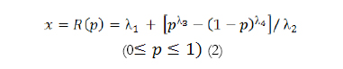
where p is a uniform random variable (0,1) and x follows the GLD. Ramberg et al. (1979) explored how to determine the distribution parameters using the first four moments, and how to fit the resulting distribution. The skewness and kurtosis of the GLD are determined by λ₃ and λ₄, respectively. Given these valúes, the variance is determined by λ₂, whereas the mean can take any valúe (λ₁).

In recent research, controversy has arisen regarding which data generation procedure is the most suitable for generating accurate non-normal distributions. The Fleishman (1978) method is one of the most widely used in simulation studies, and it has the advantage of being simple, quick and easily generalized to the generation of multivariate non-normal data, through the procedure described by Vale and Maurelli (1983). However, some authors have argued that the procedure proposed by Ramberg et al. (1979) is able to generate more extreme non-normal distributions, although when it comes to non-extreme, non-normal distributions the two procedures offer an equivalent speed and ease of execution (Tadikamalla, 1980). Likewise, other studies have pointed out that the two procedures are similar and present the same limitations when generating non-normal distributions with extreme values of skewness and/or kurtosis (Headrick & Kowalchuk, 2007; Headrick, Sheng & Hodis, 2007).

As noted above, the fit of the generated distribution to the theoretical model is a key criterion for determining the accuracy of a data generation procedure, and some studies have highlighted the importance of investigating how the number of simulations performed affects the quality of Monte Carlo studies in general (Harwell, Stone, Hsu & Kirisci, 1996; Díaz-Emparanza, 2002), and the fit of the generated distribution to the theoretical model in particular (Bang et al., 1998; Luo, 2011). Recent research has provided fairly consistent results in this regard, and it is generally accepted that more simulations means better quality (Burton et al., 2006; Diaz-Emparanza, 2002). In Monte Carlo studies the number of simulations is usually somewhere between 100 and 100000 (Burton et al., 2006), most commonly 1000 (e.g. Collier, Baker, Mandeville & Hayes, 1967; Kowalchuk, Keselman, Algina & Wolfinger, 2004), 5000 (e.g. Keselman, Othman, Wilcox & Fradette, 2004; Lix & Keselman, 1996) or 10000 (e.g. Livacic-Rojas, Vallejo & Fernández, 2006; Wilcox, 2004). However, very few studies have examined the effect of the number of simulations on the fit of the generated distribution to the theoretical model, and the results to date are inconclusive. For example, Kashyap, Butt and Bhattacharjee (2009) found that 5400 simulations were sufficient for an adequate fit to the Bernoulli distribution, while Bang et al. (1998) reported that 10000 simulations were enough to generate data from the normal distribution. However, these studies did not consider the wide range of possible distributions or the number of simulations most commonly used in Monte Carlo simulation studies. More recently, Luo (2011) examined the accuracy of the Fleishman (1978) method and took into account a wide variety of non-normal distributions with values of skewness between 0 and 1.25 and kurtosis values between 1 and 4. This study only considered a maximum of 2000 simulations, and the results show that the procedure becomes less accurate as skewness increases, and also that this number of simulations is insufficient when the degree of contamination is severe.

In light of the above, the aim of the present study was to compare the suitability of the data generation procedures proposed by Fleishman (1978) and Ramberg et al. (1979) in terms of the fit of the generated distribution to the corresponding theoretical model, with both the number of simulations and the degree of contamination of the distribution being modified. To this end, we selected a series of non-normal distributions defined by the skewness and kurtosis values most commonly found in real data. These distributions were generated by means of the two abovementioned procedures and the number of simulations was varied. Each distribution was then compared with its respective theoretical distribution, and the degree of fit was calculated according to the deviation in the skewness and kurtosis coefficients.

 

Method

The data were generated using SAS/IML, which was chosen due to it being one of the most suitable software packages for simulating data (Kashyap et al., 2009). The study variables were:

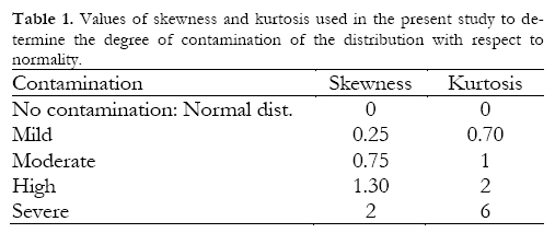
a. Degree of contamination of the distribution. The theoretical distributions selected were the normal distribution and a series of unknown non-normal distributions, defined by the skewness and kurtosis values most commonly encountered in real health and social sciences data. Blanca et al. (2013) calculated the skewness and kurtosis coefficients in 693 real data sets derived from measures of psychological variables and found, in line with other authors (Micceri, 1989), that only a small percentage of distributions were normal. More specifically, they found that skewness values ranged between -2.49 and 2.33, while those for kurtosis were between -1.92 and 7.41. Considering skewness and kurtosis together, only 5.5% of distributions were close to expected values under normality; in terms of absolute values of skewness and kurtosis 39.9% of values were between 0.26 and 0.75, 34.5% were between 0.76 and 1.25, 10.4% were between 1.26 and 1.75, 2.6% were between 1.76 and 2.25, and 7.1% were greater than 2.25. On the basis of these results we selected skewness and kurtosis coefficients that represented different degrees of contamination with respect to normality, from mild to severe. These values are shown in Table 1.

 

 

b. Type of data generator. Data were generated by means of two procedures, the Fleishman (1978) method and that developed by Ramberg et al. (1979). In the former we used the coefficients a, b, c and d for the values of skewness and kurtosis that are shown in the table of Fleishman (1978). For those values that do not appear in this table the coefficients a, b, c and d were calculated by means of a polynomial transformation in SAS, using the syntax shown in Appendix I. In order to generate data by means of the procedure proposed by Ramberg et al. (1979) we used lambda values (ta, ta, ta and ta) for the different values of skewness and kurtosis shown in the tables of Karian and Dudewicz (2000). The values of the coefficients a, b, c and d and the lambda values are shown in Tables 2 and 3, respectively.

c. Number of simulations. Data were generated for the different theoretical distributions using between 1000 and 15000 simulations (number of iterations), in steps of 1000. Subsequently, and so as to ensure that the statistical analysis was interpretable, the number of simulations was grouped into five categories: 1000-3000, 4000-6000, 7000-9000, 10000-12000 and 13000-15000.

In order to analyse the accuracy of the data generators used in the simulations we examined the fit of the generated distribution with respect to the theoretical model, calculating the differences in absolute values between the respective theoretical coefficients of skewness and kurtosis and those obtained in the generated distribution; these were labelled, respectively, the skewness deviation and the kurtosis deviation. For both variables, values of 0 indicate a perfect fit between the theoretical and generated distributions. The coefficients of skewness (3) and kurtosis (4) were calculated by means of SAS, which uses the following unbiased estimators:

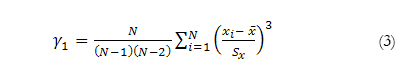
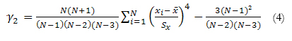
where N is the number of observations, x₁ represents the i-th value of the variable, ‾x corresponds to the mean and S_x the standard deviation.

 

Results

In order to analyse differences according to the type of data generator (Ramberg vs. Fleishman), the degree of contamination of the distribution (normal, mild, moderate, high and severe) and the number of simulations (1000-3000, 40006000, 7000-9000, 10000-12000 and 13000-15000) we conducted two 2 x 5 x 5 analyses of variance, with skewness deviation and kurtosis deviation as the dependent variable, respectively. Each cell of the design contains three observations. Table 4 shows the results of the analysis.

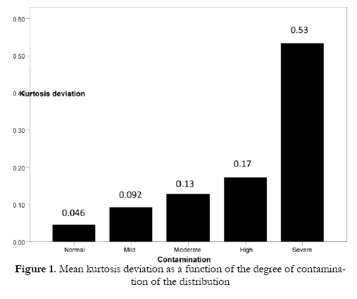
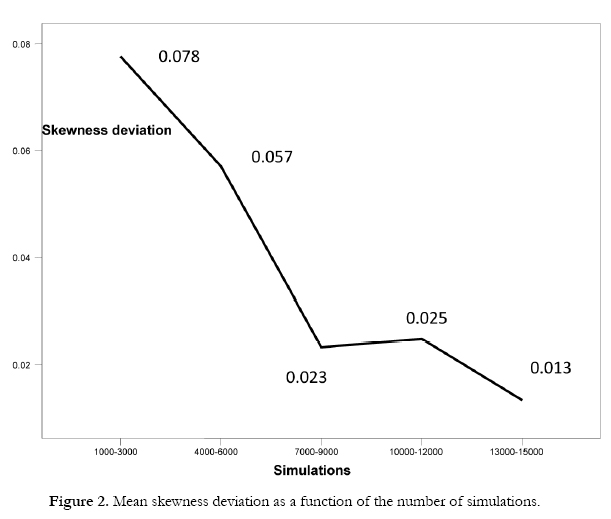
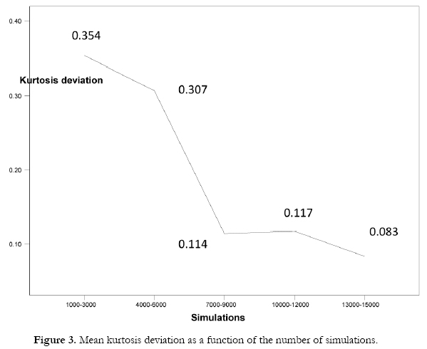
The main effects show that there are no differences between the two data generators as regards the skewness deviation or kurtosis deviation. The total mean deviation for skewness was 0.04 (SD= 0.05), while that for kurtosis was 0.20 (SD= 0.30). With respect to the degree of contamination there were differences in terms of the kurtosis deviation but not in the skewness deviation. Specifically, the kurtosis deviation increased in line with the degree of contamination, and was at its highest when the simulated distribution showed severe contamination (Figure 1). As regards the number of simulations, this was associated with differences in both skewness deviation and kurtosis deviation. In general, both deviations decreased as the number of simulations increased, with lower deviations being produced above 7000 simulations (Figures 2 and 3).

 

 

 

 

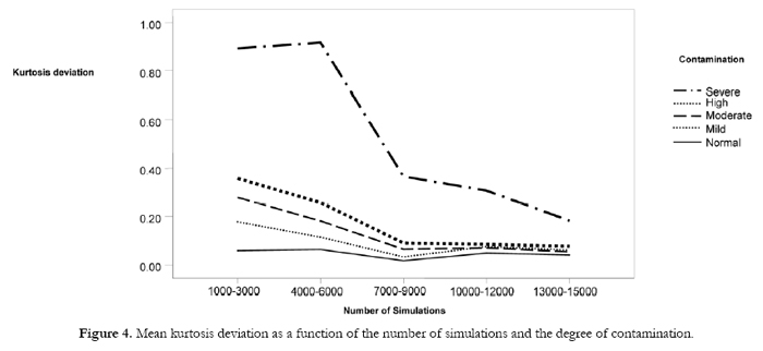
The interaction effects show that the two data generators produce a similar pattern as regards the skewness and kurtosis deviations and the number of simulations, there being no interaction between these factors. However, the kurtosis deviation as a function of the degree of contamination did vary according to the number of simulations (Figure 4). In general, the kurtosis deviation is greater with 6000 simulations or fewer, and lower above 7000 simulations for all the distributions. Note, however, that the greatest deviation occurs when simulating a distribution with severe contamination, especially when the number of simulations is less than 7000.

 

 

Discussion

The main aim of this study was to compare two data generation procedures, the Fleishman (1978) method and that proposed by Ramberg et al. (1979), as regards the fit of the generated distribution to the theoretical model, with both the number of simulations and the degree of contamination of the distribution being modified. In addition to the normal distribution we considered a series of distributions with different degrees of contamination, specifically those most frequently encountered in health and social sciences research (Blanca et al., 2013). Fit was evaluated by calculating the differences in absolute values between the respective theoretical coefficients of skewness and kurtosis and those obtained in the generated distribution.

The results show that the data generation procedure proposed by Ramberg et al. (1979) is as accurate as the Fleishman (1978) method for both normal and non-normal distributions, a finding that is consistent with previous research (Headrick et al., 2007; Headrick, Sheng et al., 2007). Both procedures also show less skewness deviation than kurtosis deviation when generating data. However, their accuracy differs as a function of the number of simulations and the degree of contamination with respect to normality. In general, as the degree of contamination of the distribution increases, so does the number of simulations required to ensure a good fit. These results confirm the findings of previous research (Burton et al., 2006; Díaz-Emparanza, 2002) which reported that increasing the number of simulations improves the quality of a simulation study, and they are also consistent with the conclusions reached by Luo (2011). Luo (2011) found that when using the Fleishman (1978) method a higher number of simulations are required as the degree of skewness in the desired distribution increases.

More specifically, one of the main conclusions to be drawn from the present study is that when deciding how many simulations are required to ensure accurate data generation it is necessary to take into account the values of skewness and kurtosis that one wishes to simulate. On the one hand, both the data generators studied here are more accurate when generating normal and non-normal distributions with over 7000 simulations, above which number the values of skewness and kurtosis deviation are close to zero. However, when the simulated distribution presents severe contamination, defined by skewness of 2 and kurtosis of 6, both procedures become less accurate and yield higher values of kurtosis deviation. In these cases the lowest deviation is produced between 13000 and 15000 simulations, where the kurtosis deviation takes a value of 0.20. Although these results cannot be directly compared with other studies, as this is the first report to compare the procedures of Fleishman (1978) and Ramberg et al. (1979) in terms of the number of simulations required to generate non-normal data, our findings are partially consistent with previous research stating that the quality of simulation studies can be increased by using 10000 simulations (Bang et al., 1998; Rasch & Guiard, 2004; Robey & Barcikowski, 1992).

In summary, the results show that the two data generation procedures behave similarly. However, as the degree of contamination of the theoretical distribution increases, so does the number of simulations required to ensure a good fit to the generated data. Future research should analyse the degree of fit with other types of known non-normal distributions that are widely used in Monte Carlo studies, for example, the double exponential or lognormal. Similarly, it would be useful to consider distributions with different values of skewness and kurtosis, with one of these being set at zero. Finally, it would also be interesting to replicate the present study with multivariate data so as to analyse the accuracy of the multivariate extensions of these two procedures.

 

References

1. Afflerbach, L. (1990). Criteria for the assessment of random number generators. Journal of Computational and Applied Mathematics, 31, 3-10.         [ Links ]

2. Bang, J. W., Schumacker, R. E. & Schlieve, P. L. (1998). Randomnumber generator validity in simulation studies: An investigation of normality. Educational and Psychological Measurement, 58(3), 430-450.         [ Links ]

3. Blanca, M. J., Arnau, J., Bono, R., López-Montiel, D., & Bendayan, R. (2013). Skewness and kurtosis in real data samples. Methodology. European Journal of Research Methods for the Behavioral and Social Sciences, 9(2), 78-84. doi:10.1027/1614-2241/a000057.         [ Links ]

4. Brown, D. D., Weatherholt, T. N. & Burns, B. M. (2010). Attention skills and looking to television in children from low income families. Journal of Applied Developmental Psychology, 31, 330-338.         [ Links ]

5. Burton, A., Altman, D. G., Royston, P. & Holder, R. L. (2006). The design of simulation studies in medical statistics. Statistics in Medicine, 25, 4279-4292.         [ Links ]

6. Claret, L., Girard, P., Hoff, P. M., Van Cutsem, E., Zuideveld, K. P., Jorga, K., Fagerberg, J. & Bruno, R. (2009). Model based-prediction of phase III overall survival in colorectal cancer on de basis of phase II tumour dynamics. Journal of Clinical Oncology, 27, 4103-4108.         [ Links ]

7. Collier, R. O., Baker, F. B., Mandeville, G. K. & Hayes, T. F. (1967). Estimates of test size for several test procedures based on conventional variance ratios in the repeated measures design. Psychometrika, 32, 339-353.         [ Links ]

8. Deluchi, K. L. & Bostrom, A. (2004) Methods for analysis of skewed data distribution in psychiatric clinical studies: Working with many zero values. American Journal of Psychiatry, 161, 1159-1168.         [ Links ]

9. Demirtas, H. (2007). Letter to the Editor: The design of simulation studies in medical statistics. Statistics in Medicine, 26, 3818-3821.         [ Links ]

10. Díaz- Emparanza, I. (2002). Is a small Monte Carlo analysis a good analysis? Checking the size, power and consistency of a simulation-based test. Statistical Papers, 43, 567-577.         [ Links ]

11. Fleishman, A. (1978). A method for simulating non-normal distributions. Psychometrika, 43(4), 521-531.         [ Links ]

12. Horner, R. D. (1987). Age at onset of Alzheimer' s disease: Clue to the relative importance of etiologic factors? American Journal of Epidemiology, 126, 409-414.         [ Links ]

13. Karian, Z. A. & Dudewicz, E. J. (2000). Fitting statistical distributions. The generalized lambda distribution and generalized bootstrap methods. Boca Raton, FL: Chapman and Hall/CRC.         [ Links ]

14. Kashyap, M. P., Butt, N. S. & Bhattacharjee, D. (2009). Simulation study to compare the random data generation from Bernoulli distribution in popular statistical packages. Pakistan Journal of Statistics and Operation Research, 5 (2), 99-106.         [ Links ]

15. Keselman, H.J., Othman, A. R., Wilcox, R. R. & Fradette, K. (2004). The new and improved two-sample t test. Psychological Science, 15 (1), 47-51.         [ Links ]

16. Keselman, H. J., Wilcox, R. R. & Lix, L. M. (2003). A generally robust approach to hypothesis testing in independent and correlated group designs. Psychophysiology, 40(4), 586-596.         [ Links ]

17. Kowalchuk, R. K., Keselman, H. J., Algina, J. &Wolfinger, R. D. (2004). The analysis of repeated measurements with mixed-model adjusted F tests. Educational and Psychological Measurement, 64(2), 224-242.         [ Links ]

18. Harwell, M. R., Stone, C. A., Hsu, T. C. & Kirisci, L. (1996). Monte Carlo studies in item response theory. Applied Psychological Measurement, 20, 101-125.         [ Links ]

19. Headrick, T. C. & Kowalchuk, R. K. (2007). The Power Method Transformation: Its Probability Density Function, Distribution Function, and Its Further Use for Fitting Data. Journal of Statistical Computation and Simulation, 77, 229-249.         [ Links ]

20. Headrick, T. C., Sheng, Y. & Hodis, F. (2007). Numerical computing and graphics for the power method transformation using Mathematica. Journal of Statistical Software, 19(3), 1-17.         [ Links ]

21. Limpert, E., Stahel, W. A. & Abbt, M. (2001). Log-normal distributions across the sciences: keys and clues. BioScience, 51, 341-352.         [ Links ]

22. Livacic-Rojas, P., Vallejo, G. & Fernández, P. (2006). Procedimientos estadísticos alternativos para evaluar la robustez mediante diseños de medidas repetidas. Revista Latinoamericana de Psicología, 38 (3), 579-598.         [ Links ]

23. Lix, L. M & Keselman, H. J. (1996). Interaction contrasts in repeated measures designs. British Journal of Mathematical and Statistical Psychology, 49, 147-162.         [ Links ]

24. Luo, H. (2011). Generation of non-normal data: A study of Fleishman's Power Method. Working paper published by the Department of Statistics of Uppsala University (Sweden). Retrieved from http://urn.kb.se/resolve)urn:nbn:se:uu:diva-150623.         [ Links ]

25. Niederreiter, H. (1992). Random number generation and quasi-Monte Carlo methods. Philadelphia: SIAM.         [ Links ]

26. Matud, P., Carballeira, M., Lopez, M., Marrero, R. & Ibáñez, I. (2002). Apoyo social y salud: un análisis de género. Salud Mental, 25(2), 32-37.         [ Links ]

27. Micceri, T. (1989). The unicorn, the normal curve, and other improbable creatures. Psychological Bulletin, 105, 156-166.         [ Links ]

28. Qazi, S., DuMez, D. & Uckun, F. M. (2007). Meta-analysis of advanced cancer survival data using log-normal parametric fitting: A statistical method to identify effective treatment protocols. Current Pharmaceutical Design, 13, 1533-1544.         [ Links ]

29. Ramberg, J. S., Dudewicz, E. J., Tadikamalla, P. R., & Mykytka, E. F. (1979). A probability distribution and its uses in fitting data. Technometrics, 21 (2), 201-214.         [ Links ]

30. Ramberg, J. S. & Schmeiser, B. W. (1972). An approximate method for generating symmetric random variables. Communications of the ACM, 15(11), 987-990.         [ Links ]

31. Ramberg, J. S. & Schmeiser, B. W. (1974). An approximate method for generating asymmetric random variables. Communications of the ACM, 17 (2), 78-82.         [ Links ]

32. Rasch, D. & Guiard, V. (2004). The robustness of parametric statistical methods. Psychology Science, 46, 175-208.         [ Links ]

33. Ripley, B. D. (1990). Thoughts on pseudorandom number generators. Journal of Computational and Applied Mathematics, 31, 153-163.         [ Links ]

34. Robey, R. R. & Barcikowski, R. S. (1992). Type I error and the number of iterations in Monte Carlo studies of robustness. British Journal of Mathematical and Statistical Psychology, 45, 283-288.         [ Links ]

35. Shang-wen., Y. & MingHua, H. (2010). Estimation of air traffic longitudinal conflict probability based on the reaction time of controllers. Safety Science, 48, 926-930.         [ Links ]

36. Soler, H., Vinayak, P. & Quadagno, D. (2000). Biosocial aspects of domestic violence. Psychoneuroendocrinology, 25, 721-739.         [ Links ]

37. Sullivan, T. P. & Holt, L. J. (2008). PTSD symptom clusters are differentially related to substance use among community women exposed to intimate partner violence. Journal of Traumatic Stress, 21 (2), 173-180.         [ Links ]

38. Tadikamalla, P. (1980). On simulating non-normal distributions. Psychometrika, 45(2), 273-279.         [ Links ]

39. Ulrich, R. & Miller, J. (1993). Information processing models generating lognormally distributed reaction times. Journal of Mathematical Psychology, 37, 513-525.         [ Links ]

40. Vale, C. D. & Maurelli, V.A. (1983). Simulating multivariate non normal distributions. Psychometrika, 48, 3, 465-471.         [ Links ]

41. Van der Linden, W. J. (2006). A log-normal model for response times on test items. Journal of Educational and Behavioral Statistics, 31 , 181-204.         [ Links ]

42. Wilcox, R. R. (2004). An extension of Stein's two-stage method to pairwise comparisons among dependent groups based on trimmed means. Sequential Analysis, 23 (1), 63-74.         [ Links ]

 

 

Correspondence:
Rebecca Bendayan
Departamento de Psicobiología y Metodología de las Ciencias del Comportamiento
Facultad de Psicología, Campus de Teatinos
Universidad de Málaga. 29071 Málaga (Spain)
E-mail: bendayan@uma.es

Article received: 10-09-2011
Reviewed: 16-11-2012
Accepted: 16-02-2013