


 Custom services
 English (pdf)
 Article in xml format
 Article references
 Send this article by e-mail
 Cited by SciELO
  Cited by Google
  Similars in
SciELO
Similars in
SciELO  Similars in Google
 Permalink
Introduction
In the past decade there has been much discussion about so-called questionable research practices (QRPs), a set of behaviors of scientists that distort the research process and bias the results (Bakker et al., 2012; DeCoster et al., 2015; Earp & Trafimow, 2015; Pashler & Harris, 2012). Many claim that QRPs are a major threat to the validity of the conclusions of research. Its consequences occur both when conducting primary research and when doing meta-analytical reviews.
Several expressions have been used to refer to the QRPs, but recently the term p-hacking (pH) has been used to describe a set of problematic practices that can lead to systematic bias in conclusions based on published research (Simonsohn et al., 2014a). One result of pH is to select those statistical analyses that lead to non-significant p-values being transferred to the region of statistical significance. In practical terms, a result that should have an associated p-value greater than the level of significance (α) ends up having a p-value below that threshold.
Beyond fraudulent behaviors, such as intentionally fabricating or falsifying data (Stricker & Günther, 2019), QRPs are psychologically more “tolerable”. They consist of means to “cook” the data by transforming them in various ways, analyzing them with several alternative statistical techniques, analyzing multiple indicators without informing readers of failed methods, performing non-programmed intermediate statistical analyses, selectively eliminating participants, etc. (Fanelli, 2009; Hall & Martin, 2019; John et al., 2012). If instead of reporting the result of the “normal” analyses, these practices are carried out with the aim of finding a p-value below α, but without informing readers of the steps taken to produce such results, these procedures inevitably produce two consequences. First, the false positives rate is inflated beyond its nominal value (Bakker et al., 2012; Ioannidis & Trikalinos, 2007; van Assen et al., 2015), and second, in global terms the results finally reported overestimate the parametric effect size (ES) (Kraemer et al., 1998; Lane & Dunlap, 1978).
We know that different types of QRP's can produce somewhat different biases (e.g., Ulrich & Miller, 2015). We are going to focus on those forms of QRP in which, in view of a marginally significant result, the researcher does not stop the analysis, but performs actions aimed at obtaining a significant result. Typically, increase the sample and reanalyze (Botella et al., 2006), or analyze sequentially with alternative statistical techniques or transformations.
The use of pH has received considerable attention in recent years, in the context of the so-called crisis of confidence in psychology (Baker, 2016; Earp & Trafimow, 2015; Pashler & Harris, 2012; Pashler & Wagenmakers, 2012; Yong, 2012). Of course, the focus has been on the biasing effects of pH on the conclusions of single studies. However, a logical extension of those worries is the concern about the potential effects on the conclusions of the meta-analyses carried out in research fields where there is a detectable pH activity. The pH activity in the primary studies could have a kind of domino effect on the meta-analyses that synthesize those studies.
We must prevent and fight QRPs for several good reasons, which we will discuss later. These arguments refer above all to the harmful effects that the results of primary studies contaminated by QRPs can have on their own as well as on the advancement of a scientific field such as psychology. However, we will argue that pH (at least the type of pH we are focusing on here) does not have an important impact on the combined estimate of ES calculated in meta-analyses. In fact, its quantitative impact on meta-analytical estimates is rather small. Our goal in this article is to support the conclusion that calculating the impact of a specific type of pH over a range of meta-analytical conditions can be demonstrated to be surprisingly small to the point of insignificance. To advance the main argument, the reason why the impact of this type of pH on the meta-analysis is small is twofold: (a) the probability that a given study has been subjected to pH such that its results are consequently modified, is relatively small, and (b) the impact of the distortion produced by those few studies in the overall estimation of the population ES is also correspondingly small.
Assessing the prevalence of pH
There are two main sources of evidence for the existence of pH: surveys of researcher practices and statistical analyses of the empirical distributions of ES estimates. Fanelli (2009) performed a meta-analysis of 18 surveys of researchers about their own behavior regarding QRPs, and about those of close colleagues. The results showed that QRPs are present in all scientific branches, with different degrees of prevalence. Unfortunately, the responses also indicate that a non-negligible number of researchers do not perceive some of these QRPs as particularly dishonest. The conclusion is clear: QRPs exist and their presence is not negligible (see, for example, the figure 1 of Brodeur, Lé, Sangnier & Zylberberg, 2016; or those of Krawczyk, 2015). However, the prevalence estimates vary widely, depending on the method used and the field and subfield analyzed (Banks et al., 2016; Head et al., 2015).
Several statistical procedures have been proposed to test for the presence of pH in a given empirical distribution of p-values. On the one hand, the transfer of p-values between regions should be visible in the form of an over-abundance of studies in the region of significant values adjacent to non-significant values (for example, .03 - .05). Similarly, in the area of p-values on the other side of the threshold (just above α; for example, .05 - .07) there must be an equivalent shortage of studies. On the other hand, we should notice an overabundance within the area of significant p-values adjacent to the threshold with respect to other more remote areas, according to the p-curve model fitted. These trends are represented in Figure 1, which shows the smoothed difference between the expected frequency of p-values within the range 0 < p ≤ .10 in the absence of pH and with a transfer of p-values from the range .05 < p ≤ .10 to the range .025 < p ≤ .05. There is an abrupt step in the threshold value of statistical significance (typically, .05). Depending on the size of the step, the practical effect of pH on the combined estimate of ES will be greater or lesser.

The effects of pH are hardly detectable in empirical distributions of p-values, since the effects of publication bias (PB) mask them (Francis, 2012). The PB against non-significant studies is another threat that biases the combined estimates of the population ES. It is a real and important threat to the validity of conclusions based on meta-analyses that has been well studied and documented for decades (Mueller, 2018; Rothstein et al., 2005; Schneck, 2018; van Aert et al., 2019). Graphically, PB produces a step in the expected distribution of p-values that can be very similar to that produced by pH. A practical difficulty in assessing the effects of pH with real databases is that, in the scientific fields in which we detect the presence of pH, a significant presence of PB is also often detected (e.g., Head et al., 2015; Krawczyk, 2015). Both factors, pH and PB, can be reflected in abrupt changes in the distribution of p-values around the threshold (Figure 1), between those categorized as significant and those that are not (typically α = .05), so that their effects are easily confused (Leggett et al., 2013). Consequently, in the calculations that follow, we assume analytic scenarios in which there is pH but no PB. In this way, we can assess the pure effect of pH. Even so, we will also see the effect of pH when meta-analytic methods are applied only to significant studies, as a way to protect against PB. We will see how large the effect of pH is on the estimation of ES when a method such as p-curve analysis is applied to the set of significant studies (Simonsohn et al., 2014b).
Several studies have assessed the presence of pH in the literature. Head et al. (2015) used data mining techniques to extract distributions of p-values from a variety of scientific fields, and they concluded that pH effects are pervasive (but see Hartgerink, 2017). Brodeur et al. (2016) estimated that in the field of economics there is a transfer of between 10% and 20% studies from the area of marginally significant to that of significant.
The analysis of the p-values reported in more than five thousand articles in experimental psychology journals reported by Krawczyk (2015) reveals several interesting features. Of course, there are anomalies in the empirical p distribution. However, along with an over-abundance of values that are significant but close to the limit of that region (for example, below .05 but close to it), there is also an even greater over-abundance of values above but also very close to the threshold of significance (for example, above .05 but close to it). The interpretation of this pattern is not clear. However, since these anomalies could be due to several factors, especially PB, they seem to indicate that pH as such should have had a rather small incidence in the observed distribution of p-values (see Krawczyk, 2015, Figures 3 and 4).
Bishop and Thompson (2016) have studied the presence of anomalies in p-value distributions through simulations and a re-analysis of the data by Head et al. (2015). They conclude that neither the absence of a bump in the p-curve is indicative that there is no pH, nor is its presence undoubtedly associated with a distribution contaminated by p-values from a nongenuine origin. To reach a sound conclusion, you must assume a specific QRP. In their work they focus on what they call ghost variables, which translate into the parallel analysis of various outcome variables, reporting only the one that is most favorable to the researcher's hypothesis. This form of QRP is very difficult to detect.
Although these studies provide evidence of the presence of pH, and some even estimate its prevalence, most of them do not calculate its quantitative impact on the meta-analytical combined estimate of the ES. They only assess distribution anomalies by testing the null hypothesis of non-pH. Simonsohn, Nelson and Simmons (2014a) concluded that it is very unlikely that in a wide range of credible conditions pH is able to yield a non-existing effect. We believe that we must go beyond knowing how probable it is that pH turns a null effect into an incorrect, non-null effect. We want to calculate the impact of a specific type of pH on the combined estimation of ES to know how much we should worry about its biasing effects when assessing the results of a meta-analysis. Specifically, the type of pH that consists of selecting those statistical analyses that lead to p-values in the region sometimes referred to as "marginally significant" being transferred to the region of statistical significance1. As we have already suggested, our hypothesis is that although we must protect our research and actively fight pH for several reasons, the estimated effect of this specific type on the combined estimation of the ES in meta-analysis is very limited.
Method
In what follows we have limited ourselves for simplicity of exposure to one-sided tests with α = .05 and a normally distributed test statistic. All arguments generalize to two-sided tests and to other values of α. Likewise, we have assumed that all studies have the same sample size. Of course, in real research, the sample sizes vary among the studies, but by assuming equal sizes we simplify the calculations without affecting the conclusions. To calculate the effect of pH on the ES estimation we used a linear combination of the expected values of the test statistic, conditionalized on specific ranges of values obtained in the statistical test. For example, if the statistic tested under the null hypothesis follows a normal distribution, we can obtain its expected value conditionalized on being less than 1.645 (not significant; p > .05) and on being equal to or greater than 1.645 (significant; p ≤ .05). If we also know the probabilities that the values fall within each of these regions, the total expected value can be obtained by weighing the partial expected values with their corresponding probabilities. The expected conditionalized values are easily obtained from the truncated normal distribution (Johnson, Kotz, & Balakrishnan, 1994, chap. 13). Specifically, the expected value of the test statistic, T, is,

Let's see a simplified, non-realistic example of how we are going to do the calculations, with only two regions, although in the real calculations later we will define a more complex and realistic scenario. If, for example, we randomly transfer studies (with a probability of .50 that a study is transferred) from the region with p > .05 to the region with p ≤ .05, the expected value after these transfers is obtained by recalculating the weights (probabilities) of the conditional expected values. In order to assess the effects of pH in terms of transfers of observations between regions (Figure 2), we will also make two instrumental assumptions. The first states that the probability of transferring a specific study from one region to another is uniform within the region of origin. That is, the probability of transferring, through QRPs, an observation with a p-value of (say) between .05 and .10, is the same for all studies performed while p is within that range.
The second instrumental assumption states that when transferring studies with .05 < p ≤ .10 to the region with .025 < p ≤ .05, the expected value of T is approximately the same as that for studies with genuine p-values in that region. These two instrumental assumptions are set to facilitate calculations. Moderate deviations from them do not generate large differences in the results, whereas other approaches require rather arbitrary assumptions.
In Figure 2 we see that the values that define several regions in the right tail of the distribution of the test statistic under the null hypothesis also define different regions in the true distribution, which is that to the right (with δ > 0). If we operationally define pH as a transfer (represented by the arrow) of cases from the “marginally significant” region to the “significant” region closest to the significance threshold, we can calculate the expected value of the test statistic and, therefore, the bias produced by a pH of such magnitude. Specifically, we have assumed that there is a probability, q, that a value in the region defined as .05 < p ≤ .10 (that is, 1.280 ≤ T <1.645) is transferred to the region .025 < p ≤ .05 (that is, 1.645 ≤ T <1.96). We have calculated the effect of these transfers with conditional probabilities of up to q = .50. This implies a maximum in which half of the results with marginally significant p-values end up being significant after being submitted to QRPs. The percentage of exploratory studies submitted to QRPs may be higher, but only a part (up to 50% of those judged to be marginally significant in our calculations) end up being reported with a statistically significant p-value. We believe that even this estimate is high and that in real contexts it is probably smaller than this maximum (Banks et al., 2016; Fanelli, 2009; Fiedler, Schwarz, 2016; John et al., 2012; Martinson et al., 2005). For example, in their analysis of research published in the field of economics Brodeur et al. (2016) estimate that those transfers represent between 10% and 20% of marginally significant studies. A survey by Martinson, Anderson and De Vires (2005) found that the self-reported frequencies of incurring QRPs are typically less than 15%. In other analyses, it is assumed that 100% of the nonsignificant studies are subjected to pH (Simonsohn et al., 2014b), a prevalence that seems exaggerated 2.

Figure 2. Regions for the statistical test value under the null (left curve) and under the true value (right curve) hypotheses. The letters represent the four regions of the true distribution: A (not significant), B (marginally significant), C (significant with high p) and D (significant with low p). The arrow represents the transfer of studies with marginally significant p values to the region with significantly associated p values but close to the threshold defined by α.
We have worked with Cohen's d as our effect size index, with two sample sizes that reflect a typically small size in psychology (two groups of 15) and a typically moderate size (two groups of 30) (Marszalek et al., 2011; Rubio-Aparicio et al., 2018). With larger samples, the effects of pH tend to be even smaller.
The δ values selected (besides 0 for non-effect) are 0.2, 0.5 and 0.8, generally used since Cohen (1988) to designate small, moderate and large standardized mean differences (see also Rubio-Aparicio et al., 2018).
Let us see with a detailed example how we have performed our calculations in the condition with δ = 0.80 and N = 15 (see in Appendix S1, supplemental material, the R syntax that allows to reproduce the calculations reported for this and all other conditions). The expected conditional values have been obtained through the truncated normal distribution. The probability that a study yields a result that is neither significant nor marginally significant (T < 1.28; region A in Figure 2) is .1904, and the expected value of T for that set of studies is 0.708. The probability and the expected value of significant studies with p ≤ .025 (region D in figure 2) are .5879 and 2.879, respectively. These two sets of studies are those not affected by the transfer represented by the arrow in Figure 2. The probability that in the test of the null hypothesis, the T value is in the region of "marginally significant" (1.280 ≤ T <1.645; region B in Figure 2) is equal to .1093, and its expected conditional value is 1.47. Finally, the probability that the p-value remains in the region of significant values with high p-values (.025 < p ≤ .05; region C in Figure 2) is equal to .1124 and the conditional expected value of T is 1.806. The total expected value of T in the absence of pH would be:

Of course, the expected value of d is E(d) = E(T)·sqrt (2/N) = 2.1911·sqrt(2/15) = 0.800. Let us now see what happens in this body of research if the magnitude of pH is set to 50% of the marginally significant studies (q = .5), becoming significant with high p-values (between .025 and .05). Half of the studies within that range of p-values (.1093 / 2 = .0546) are transferred to the adjacent area (region C). The expected value of T with that level of pH is:

Then, E(d) = 2.2093·sqrt(2/15) = 0.807. The magnitude of the bias produced by this degree of pH in this analytic scenario is 0.807 - 0.800 = 0.007.
Results and discussion
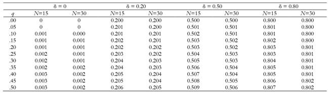
Table 1 shows the main results in terms of the expected values of d for the different conditions. In each case, the bias is the difference between the value within the table and the true value of δ. In all conditions the bias is less than one hundredth: │E(d) - δ│ < 0.01. The greatest biases occur with the smallest sample size (N = 15). The magnitude of the bias effect is generally small and, in many conditions, negligible (less than ± 0.005). We can state that pH is not likely to have a relevant quantitative impact on the estimation of ES, at least for the conditions studied here. It is easy to understand the two reasons why the impact is small. On the one hand, the probability that a study is subject to QRPs, and the results transferred from the region of marginally significant (region B) to a significant one with high p-values (region C, p-values between .025 - .05), is small. On the other hand, the conditional expected values of the test statistic in those two adjacent regions are very close. Let us return to the example with δ = 0.80 and N = 15. The probability that a value of T falls in the region of “marginally significant” (1.280 ≤ T <1.645) equals .1093, so the maximum transfer we have contemplated (q = .50) would eventually be, in the long run, only 5.46% of the studies carried out. These transferred studies would have a mean value of T = 1.47 (d = 0.54) in the long run before being subjected to pH, while after that process their average value would be T = 1.81 (d = 0.66). However, the vast majority of studies (in the long run 100 - 5.45 = 94.54%) would not change their associated values of T (and d).
Generalizing to other conditions
We want to know whether our conclusion is valid only for the conditions studied until here, and whether it will change significantly in other analytic scenarios. We review the main factors that could affect the conclusions and discuss their potential effects.
(a) Values of δ. The ES values chosen for δ are those that Cohen proposed as typically small, medium and large ESs. They cover a wide range of representative values of the effects studied by psychologists (Bosco et al., 2015; Richard et al., 2003; Rubio-Aparicio et al., 2018). As the bias reduces from when δ equals 0.50 to 0.80, the tendency is that with values greater than 0.80 the bias will be even lower.
(b) Sample size. Sample size does not seem to be a relevant factor, since with N = 15 and N = 30 the results are very similar. With N > 30 the results will be very stable and will show even smaller biases. It is possible that with groups smaller than 15 there is a greater difference, but these sample sizes are not very frequent in psychology, and when they are used, the data are often analyzed with non-parametric techniques. Even so, we have made the calculations with δ = 0.50 and two groups of N = 10. The results are essentially the same, reaching one hundredth of bias only when q = .50.
(c) The effect size index. Our calculations refer to δ, the standardized mean difference. We ask ourselves whether the conclusions are generalizable to other ES indices. We have made the calculations assuming that the test statistic is normally distributed, so they should be similar for other statistics that have approximate normal distributions. To calculate the bias with other indices, we simply use the corresponding formulas. For example, for Pearson's correlation we have used the values suggested by Cohen for a small, medium and large correlation (rho = .10, .30, and .50; see also Richard, Bond, & Stokes-Zoota, 2003) transformed to Fisher's Z and with samples of size 15 and 30. The results appear in Table S1 (tables S1 to S6 are included in the supplemental material). In all conditions the bias is less than one hundredth, │E(r) - ρ│ < 0.01. In the majority they are less than half a hundredth, although to reach that value the percentage of transfers must reach 50% and the sample must be small (N = 15). Therefore, we can generalize our main conclusion to r as the ES index: the quantitative impact of pH over a wide range of credible conditions is also very small for Pearson's correlation, and is negligible in practical terms.
(d) The statistical model. We have made our calculations for simplicity under a fixed effect model, although psychologists rarely use it. The random effects model is generally considered more realistic (Borenstein, Hedges, Higgins, & Rothstein, 2010). In order to show that our main result does not depend on the assumed model, we have performed a Monte Carlo simulation (see the syntax code in appendix S2 in the supplemental material). We have generated 100,000 samples for each condition. For the conditions, we have defined four mean ES values (0, 0.20, 0.50, and 0.80) and three representative variance values (0.05, 0.10, and 0.15) (Rubio-Aparicio et al., 2018). By crossing the 12 conditions with the same pH levels as in the other sections, we have obtained the results of table S2. As can be seen, the levels of bias are still very low; in no case does the mean bias reach one hundredth.
(e) Broadening the operational definition of marginally significant. We have defined pH as illegitimate transfers of results from the region in which .05 < p ≤ .10 to that of .025 < p ≤ .05. We believe this is a reasonable operationalization of pH, but one could ask how much the bias will change if we extend it, for example to the region of .05 < p ≤ .20 (i.e. 0.84 ≤ T <1.645). Table S3 shows the level of bias obtained with this new operational definition of pH. Beyond the modification in the operational definition of "marginally significant", the rest of the conditions are the same as in the calculations in Table 1.
With such a broad definition of pH, we obtain again small levels of bias. The bias exceeds two hundredths only in a few conditions, especially with small samples (N = 15) and high percentages of transferred studies (q > .30). Only in one of the conditions does it reach three hundredths (δ = 0.50; N = 15; q = .50).
(f) Variations in the sample sizes. To facilitate the calculations, we have assumed that the sample sizes of the studies are constant (N = 15 or N = 30), arguing that if they were variable, the results would not change significantly. In order to avoid any doubt in this regard (and following the suggestion of a reviewer) we have used a simulation methodology to recalculate the bias in such circumstances (see supplemental material). Specifically, we have generated 100,000 samples for each condition, associating to each one a random sample size, following the distribution proposed by Rubio-Aparicio et al., 2018). As expected, the results (Table S4) show that the size of the bias does not depend on whether the sample sizes vary. With variable sample sizes the bias is still very small.
(g) The meta-analytical strategy. The pH has been studied through empirical distributions of ES estimates, probably already affected by PB. This has probably led to thinking of it more in terms of the combined effect of both factors than in the isolated effect of pH. When PB exists and we ignore it, the combined estimate may suffer significant distortions (e.g., Carter, Schönbrodt, Gervais, & Hilgard, 2019). An efficient strategy to avoid the effects of PB is to analyze only significant studies, if a reasonable number of these are available (Simonsohn et al., 2014a; van Assen et al., 2015). It is assumed that PB increases the frequency of studies with non-significant results that remain in the file-drawer but does not affect the number of significant ones. Therefore, we calculate also the effect that pH, as we have defined it, would have on combined estimates that are carried out under the strategy of including only significant studies, such as with the p-curve method.
We have used the function of the p-curve generated from a statistical test normally distributed (Ulrich & Miller, 2018, equation 7), restricted to the range of significant p values (left half of Figure 1, without pH). We have recalculated the density of each value under different probabilities of transferring a result with a p value between .10 and .05 to the region between .05 and .025 (again with values of q from 0 to .50). With the new densities, we have fitted a curve with the same function. The values of the parameters thus obtained for different values of q appear in Table S5. It is clear that the bias can be very large, especially when the effect is null or small. Figure 3 shows the effect of pH when fitting a p-curve. The original function is that of the left segment drawn with a continuous line. The pH is reflected in the increase in heights in the right segment. When we take the two segments and force a fit using a function like the original by least squares, the result is that of the figure drawn with a dashed line. This function appears above the original, before the effect of pH. As Simonsohn, Nelson and Simmons pointed out, the effect of pH when using p-curve is an underestimation of the parametric effect size.
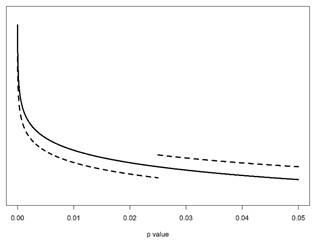
Figure 3. Effect of pH when fitting a p-curve. The dashed line (distribution of p values with pH) is divided into two segments. The one on the left is not affected by pH; the one on the right is elevated due to the transfer of p values (pH). The solid line represents the fitted function that provides the p-curve from the two segments together.
In summary, in this section we have shown that by changing the analytic scenario in several ways, the size of the bias remains small, and in most conditions it is negligible. It only increases appreciably when we extend the operational definition of "marginally significant" to the threshold p ≤ .20. On the other hand, it is much larger when using p-curve with only significant studies. Our conclusion is that the quantitative impact of this type of pH on the combined estimate of ES is generally small when the whole distribution is modeled. It is possible that in special circumstances the pH affects the empirical distribution of the ES values in a given body of studies more than in the scenarios analyzed here. However, in the vast majority of situations that we can realistically imagine, the impact is very small. To achieve a greater bias, we would have to assume much exaggerated conditions. For example, with δ = 0.50 and N = 15 even if the percentage of marginally significant studies that end up being significant as a result of pH were 100%, the bias would still be less than 0.02. A bias of five hundredths, │E (d) - δ│ = 0.05, could be achieved, for example, if the marginally significant condition is extended to studies with .05 < p ≤ .30 (i.e., 0.52 ≤ T <1.645) and it is assumed that 50% of these studies are converted to significant p-values through QRPs. These conditions involve a massive use of QRPs, which we do not believe realistically represent their prevalence in psychology.
Comparing the magnitude of the effects of pH and PB
Our main conclusion is that the magnitude of the effect of pH is generally small. Of course, the label "small" is ambiguous; we have not defined operationally a priori what a "small" bias is. In most of the conditions analyzed, the bias is less than one hundredth. The indices of ES analyzed, d and r, are often reported to two decimal places. Then the smallest possible difference due to the effect of any factor is one hundredth (and a bias smaller than ±.005 is negligible). That is why one hundredth is the unit of measure when evaluating our results. However, in order to assess the effects of pH in relative terms we have made an additional analysis, comparing the quantitative effects of pH with those of PB, the main threat in meta-analysis. We have calculated the quantitative impact on the combined estimation of the ES when there is no pH, but there are different degrees of PB and we ignore its effects. Table S6 shows the size of the bias when a proportion of non-significant studies is censored (they remain in the file drawer). For example, in the condition with δ = 0.50 the bias that occurs when half of the non-significant studies remain in the file drawer (s = .50) is much greater than that produced by pH. This is a realistic imputation of the publication rate of non-significant studies. If in this scenario the probability that the study provides non-significant results is .607 with N = 15, and, for example, 40% of them are censored, approximately one in every four studies carried out will remain in the file drawer (a very realistic situation; see, for example, the estimates of Franco et al., 2014). In this scenario, the expected value of d is 0.575. Comparing this level of bias with those of Table 1 for each condition, the conclusion is clear that the bias produced by PB (as defined here) is much greater than that produced by pH (as defined here).
Some good reasons for preventing and fighting pH
All our arguments lead to the conclusion that the magnitude of the impact of the type of pH we have focusing here on a meta-analysis when calculating combined estimates in a wide range of realistic situations is very small, even negligible. Of course, it is much smaller than the impact of PB of credible size. However, we do not want to convey the message that we can stop worrying about this type of pH. Quite the opposite. In the previous section, we have explained the reasons why we believe that it is not necessary to worry very much about its impact on the combined estimates of the ES obtained by the meta-analyst. Nevertheless, pH has other consequences, especially when assessing the results of primary investigations by themselves. We present some good reasons why we should worry about and prevent pH:
(a) The researcher crosses the line of scientific ethics, turning his or her work into a game in which opportunistic behaviors are put to work for personal gain in terms of career advancement. They reverse the priorities, putting personal profit ahead of the progress of knowledge acquired through a rigorous application of the scientific method (DeCoster et al., 2015). From a qualitative perspective, any prevalence of QRPs will be always too much. Furthermore, it is worrying that the presence of cues of QRPs is increasing, probably because the pressure to publish has been growing in the last two decades (De Winter & Dodou, 2015; Holtfreter et al., 2019; Leggett et al., 2013).
(b) A falsely significant result may be confusing for other researchers, encouraging hypotheses without sufficient support that justifies following them with new research, thus wasting time and resources.
(c) The presence of QRPs reduces the confidence of researchers in previously published results. Science should be a cooperative task of honest collaboration among scientists. If this confidence is impaired, researchers feel the need to test the results of other researchers before accepting them as valid, wasting their time and investing additional resources unnecessarily.
(d) The same happens to professionals who could apply the advancements provided by scientists. They can reduce the amount of transfers to their professional practices if they do not fully trust the process that led to the conclusions (including results that are true and useful).
(e) If QRPs are present and the society knows it, then public confidence in the value of science is eroded, and faith in scientific contributions is tainted to the extent that public policy is less influenced by research into significant problems like global warming, environmental contamination, and species extinctions (Anvari & Lakens, 2019).
(f) Confirmatory bias must be actively fought, rather than encouraged. Many young researchers normalize QRPs without being aware of being influenced by confirmatory bias. Deep inside the human mind rests the idea that our perception is more objective than that of others (Ross, 2018) and from there it easily progresses to the idea that our perceptions and intuitions are more credible than our own data. In the end, QRPs are cynically justified as acceptable behavior for the sake of scientific progress. The need to confirm previous beliefs, plus poor methodological and statistical training, within a social context in which "alternative truths" and "alternative facts" are accepted and normalized, can lead researchers to believe that what they do is correct.
(g) Incorrect conceptualizations of research methodology and statistics can be perpetuated. For example, by fostering the belief that the use of small samples makes research more efficient in terms of speed of publication, or attaching exaggerated importance to the observation that p < α. Researcher's ritualized behaviors can lead to incorrect interpretations, and the QRPs feedback those behaviors and pervasively reinforce their ritualization.
In summary, the arguments along this paper should not lead us to the conclusion that pH is not a big problem for science and that we can therefore ignore it. It has serious consequences, especially at the level of primary studies. Those consequences justify implementing measures to prevent it (e.g., Botella & Duran, 2019; De Boeck & Jeon, 2018; Marusic, Wager, Utrobicic, Rothstein, & Sambunjak, 2016; Sijtsma, 2016; Simmons, Nelson, & Simonsohn, 2011). These resulting corrective proposals are promising. Extending their implementation will not only have a positive effect on scientific methodology alone. The mere fact that the society knows that the scientific community has been alerted to potential problems and is more diligent in improving methodological rigor will be an undoubted deterrent to reduce the prevalence of QRPs.
On the other hand, not all practices labeled as QRPs are always bad practices. Using a label with such a negative load can also be confusing. For example, performing interim analyses of the data collected so far and deciding whether to continue adding participants according to the result, is not a bad practice by itself and could be more efficient. It is only a bad practice if the researcher does not disclose what has been done, and if it is done outside of some regulated procedure. We know regulated ways to do partial analyses, so that the rate of type I errors is not inflated (e.g., Botella et al., 2006). Other types of pH, as analyzing the data in unexpected ways, is a source of discovery of unexpected patterns that enriches the process of science development (Wigboldus & Dotsch, 2016). If we eliminate these unscheduled analyses from the practices of scientists, much of what their creativity can contribute is lost. What is a QRP is not to do these analyses, but not to report their exploratory nature.
Limitations
It can be argued that our way of modeling pH is somewhat limited. Surely different QRP‘s have different effects. Sequential sampling and analysis (Botella et al., 2006) influences the p-curve in a different way to the parallel analysis of multiple dependent variables and the selection of the significant ones (Ulrich & Miller, 2015), or to the application of various statistical techniques and reporting only the one that provides the most convenient value (e.g., Francis, 2012). Certainly, our way of modeling pH is very close to the first of these QRP's, which seems to be one of the most frequent in some fields of psychology. It would be necessary to study other scenarios focused on other QRP's, or even scenarios in which several or all are present at different rates.
We have focused on the impact of pH in the absence of PB. In other recent studies, the focus has been on the combined impact of both effects, especially on their interaction (e.g., Carter et al., 2019; Friese & Frankenbach, 2019). We believe that the scenario studied by us is interesting by itself. The argument for their combined study would be that it is more realistic, since both problems, pH and PB, are likely to be present in a particular field. Furthermore, it is sometimes argued that it is the presence of PB that encourages QRP's as a means of getting a study published. This being true, we believe there are other motivations for pH. Many authors feel a certain intellectual, and even emotional, commitment to certain explanatory positions and models. Personal involvement with theories can also push QRP's in fields where there is no noticeable PB, where a non-significant result would have been published anyway.
Furthermore, the fights against pH and PB are of a very different nature. We can implement mechanisms to achieve some control a priori of the studies, or plan massive replications, to avoid PB. We can also use subsequent analytical strategies that allow us to estimate and correct potential bias. However, QRP's are very difficult to control and their effects are difficult to correct. They often occur in the private domain of the researcher, or in his circle of trust. Our results at least show that if we can control and correct the PB, then we will not have to worry much about the quantitative impact of pH on the meta-analytical estimation. Our main message is that in the absence of PB the effect of pH in the meta-analytical combined estimate is very small. Therefore, an efficient strategy to improve the scientific practices is to concentrate our efforts on PB. That said, we must not forget that the small magnitude of the bias we have calculated can become a much larger bias under more extreme (although less frequent and realistic) conditions.
We have assumed two instrumental assumptions in our calculations. None of them has an empirical basis. The alternative to the first assumption would be to assume that within studies with marginally significant results, the probability of being subjected to pH is greater the lower the p-value. However, any non-uniform function would be arbitrary, and the ones we have tested have not produced very different results. Even so, it is pending to try with some different functions. The alternative to the second assumption would be to assume that the new values, after the transfer to the region of significant ones, are distributed in such a way that the conditioned expected value changes. Any specific function would be arbitrary and, again, the ones we have tested have not produced very different results. A systematic study of these alternative functions is pending. But we do not believe that reasonable deviations from these assumptions will significantly change the results.
Conclusions
QRPs are a threat to the fairness when implementing the scientific method in practice. We must fight them for several good reasons. However, our main conclusion is that among these reasons is not that they have a great impact on the meta-analytical estimation of ES. Our calculations lead to the conclusion that their real quantitative impact in a wide range of credible meta-analytical conditions is small.
Several consequences derive from this conclusion. First, researchers should not use the detection of pH as a speculative argument to justify deviations from the expected results. When they find deviations from what they expect larger than 0.02 - 0.03 in terms of d or r, they will need alternative explanations to the mere speculation that the source of the deviation could be pH without providing evidence that indeed it is.
A second consequence is that the selection models for the study of PB do not need to include additional complications derived from this practice. Modeling PB is a complex task that requires considering multiple sources of distortion in the distribution of ES values (Hedges & Vevea, 2005; Rothstein, Sutton, & Borenstein, 2005). Our results show that pH is not in general a problem that we need to take into account in the development of the models, thus avoiding unnecessary additional complexities when modeling PB.

