


 Servicios personalizados
 Inglés (pdf)
 Articulo en XML
 Referencias del artículo
 Enviar articulo por email
 Citado por SciELO
  Citado por Google
  Similares en
SciELO
Similares en
SciELO  Similares en Google
 Permalink
Introduction
Scientific researchers are faced with ever more sophisticated and innovative data analysis strategies. A good example of this is the generalized linear mixed model (GLMM), a flexible analytical strategy that has evolved from other simpler mathematical models and which has been increasingly used in recent decades. The general linear model (GLM) is the most commonly used approach in the health and social sciences (Blanca et al., 2018), where researchers often perform regression analysis, analysis of variance, and analysis of covariance. These tests require the fulfillment of a series of assumptions such as a quantitative response variable, normally distributed data, homogeneity of variance, and independence of errors, assumptions that are not always satisfied with real data. The linear mixed model (LMM) is an extension of the GLM that allows both fixed and random effects, and it is particularly useful when data are not independent (e.g., hierarchical data, repeated measures) and homogeneity of variance is not required; robust procedures for dealing with non-normality when using this model have also been developed (Arnau et al., 2012, 2013; Livacic-Rojas et al., 2010). Another extension of the GLM is the generalized linear model (GLIM), which is useful for non-normally distributed data (e.g., binary, multinomial, ordinal, count, etc.) and which fits data with an exponential family distribution through the use of non-linear link functions. Finally, the GLMM offers a more flexible approach to the analysis of data with a non-normal distribution (Bolker et al., 2009; Breslow & Clayton, 1993). The GLMM is a combination of the LMM, which includes random effects, and the GLIM, which uses different link functions that transform the expected value and the linear predictor to the same scale. In summary, each of the aforementioned models has different purposes and is suitable for specific types of data.
Empirical evidence shows that in the fields of health, education, and social science it is very common for data to be non-normally distributed (Arnau et al., 2013; Arnau et al., 2014a, 2014b; Bauer & Sterba, 2011; Blanca et al., 2013; Bono et al., 2017; Lei & Lomax, 2005; Micceri, 1989), or for there to be non-independence of observations due to nested sampling or repeated measures (Bandera & Pérez, 2018; Casals et al., 2014; Coupé, 2018; Johnson et al., 2015; Thiele & Markusen, 2012). These situations, which are very frequent in applied research, occur when repeated measurements are obtained from the same subjects (Baayen et al., 2017; Dang et al., 2008; Noh et al., 2012; Thiele & Markusen, 2012), as in the case of longitudinal studies (Bandera & Pérez, 2018; Cho & Goodwin, 2017; Fieberg et al., 2010; Koh et al., 2019; Mowen & Culhane, 2017), or when data are hierarchically structured (Casals et al., 2014; Elosua & De Boeck, 2020; Moscatelli et al., 2012; Mowen & Culhane, 2017). The fact that these situations are so common is a primary reason for using the GLMM in applied research; additionally, it is one of the alternatives to analysis of variance for repeated measures designs when the dependent variable is categorical. Use of the GLMM for multilevel models and repeated measures are further discussed in Stroup (2013).
With non-normal distributions the GLMM uses different link functions. The most frequently used link functions are logarithmic (the linear predictor is the natural logarithm of the expected value), logit (the linear predictor is the inverse of the logistic distribution function of the expected value), and probit (the linear predictor is the inverse of the standardized normal cumulative distribution function of the expected value). The most common estimation method in GLMM is the maximum likelihood (ML) procedure, especially in the form of variants such as restricted maximum likelihood (REML), restricted subject-specific pseudo-likelihood (RSPL), and penalized quasi-likelihood (PQL). Other estimation methods are the Gauss-Hermite quadrature (GHQ), the Laplace approximation (which is a particular case of the GHQ), hierarchical likelihood (HL), and Bayesian methods based on the Markov Chain Monte Carlo (MCMC) technique. The algorithm used by the GLMM allows calculation of the best linear unbiased estimator (BLUE) of the fixed effects and the best linear unbiased predictor (BLUP) of the random effects, which shows the lowest root mean square error among all the unbiased linear predictors (Bandera & Pérez, 2018; Searle et al., 1992).
These estimation methods use very complex calculation procedures that require increasingly sophisticated statistical software, such as proc glimmix in SAS, which generalizes two other procedures: proc genmod, by including error terms that are not normally distributed, and proc mixed, by considering random effects in the model (SAS Institute, 2013). Proc glimmix is a powerful technique for modeling correlated binary outcomes (Dang et al., 2008). By default, SAS uses the RSPL approach for parameter estimation (Wolfinger & O'Connell, 1993). The RSPL approach estimates random effects models based on residual probability, and it is well suited to situations where what is of interest is the individual response rather than the population mean or marginal model.
The incorporation of newer procedures into the main statistical software packages (SAS, R, STATA, and IBM SPSS) has encouraged the use of GLMMs in a wide variety of disciplines, including biology (Bandera & Pérez, 2018; Thiele & Markussen, 2012), ecology and environmental sciences (Bolker et al., 2009; Johnson et al., 2015; Kain et al., 2015; Smith et al., 2020), medicine (Brown & Prescott, 2006; Casals et al., 2014; Cnnan et al., 1998; Platt et al., 1999; Skrondal & Rabe-Hesketh, 2003; Witte et al., 2000), psychophysics (Moscatelli & Lacquaniti, 2011; Moscatelli et al., 2011; Moscatelli et al., 2012), psycholinguistics (Baayen et al., 2008; Coupé, 2018; Elosua & De Boeck, 2020; Quené & van den Bergh, 2008), and psychology (Aiken et al., 2015; Bono et al., 2021; Cho & Goodwin, 2017), among others.
Focusing on the field of psychology, Bono et al. (2021) observed a growing trend in the use of these analytic models, with the number of GLMM-related articles published in 2018 (n = 88) being more than double the figure for 2014 (n = 39). Bono et al. (2021) also carried out a systematic review of 80 empirical articles indexed in JCR journals during 2018, and which included a total of 118 different GLMM analyses. The results showed that the most common application of GLMMs involved the use of repeated measures designs (61.1 %), with two and three repeated measures (33.33 % and 25 % of analyses, respectively), and a sample of fewer than 500 participants (57.6 %). Regarding the characteristics of response variables, the most frequent among the studies analyzed were variables with two response categories (87.7 %). The most common distribution used was the binomial distribution (19.5 %), although in the majority of studies the distribution was not specified (52.5 %). Regarding software, SAS was the most widely used (36.4 %), with glimmix being the most common procedure (32.6 %).
More generally, the GLMM has most frequently been applied in longitudinal studies or repeated measures designs with binary response variables (Bakbergenuly & Kulinskaya, 2018; Cho & Goodwin, 2017; Gawarammana & Sooriyarachchi, 2017; Zhang et al., 2011), with count response variables (Coupé, 2018; Huang et al., 2016; Kruppa & Hothorn, 2021; Sun et al., 2019; Zhang et al., 2012), with multinomial outcomes (Jiang & Oleson, 2011) or, to a lesser extent, with continuous response variables (Lo & Andrews, 2015). It is worth noting that binary repeated measures are a common occurrence in biology, medicine, psychology, and sociology, as well as in many other practical fields (Gawarammana & Sooriyarachchi, 2017). These repeated measures are often related to each other, and it is common practice to use a first-order autoregressive covariance matrix, AR(1), to describe this serial dependence. Although the GLMM can model serial dependence between repeated binary responses, its use has not been widespread. Cho et al. (2018) show examples in the literature with binary time series and illustrate the GLMM AR(1) using empirical data.
Although, as we have said, GLMMs are now increasingly used by researchers in many fields, the robustness of these models has not been studied to the same extent as is the case for the LMM (e.g., Arnau et al., 2012; Jacqmin-Gadda et al., 2007; Kowalchuk et al., 2004; Vallejo et al., 2008). Indeed, simulation studies on the robustness of GLMMs with repeated measures and binary data are still very scarce. For data of this kind, Fang and Louchin (2013) found that GLMMs hold Type I error rates better than does the GLM, while Gawarammana and Sooriyarachchi (2017) concluded that the GLMM was satisfactory with respect to Type I error for sample sizes above 20.
A further issue to consider is that the results of simulation studies may be of little use to applied researchers in the psychological field, because the manipulated variables and their values (e.g., sample size, number of groups, number of repeated measures, correlation values, etc.) usually vary from one study to the next and are unlikely to have been chosen based on research practice; consequently, the results may not be directly applicable by researchers in this field. In addition, a standard criterion has not been used when assessing robustness, leading to different interpretations of the Type I error rate (Blanca et al., 2017, 2018). In this respect, the robustness of the GLMM has generally been interpreted in terms of how close or far the empirical alpha value obtained is from the nominal alpha value (Barker et al., 2017; Gawarammana & Sooriyarachchi, 2017; Zhang et al., 2012).
In this paper we report a simulation study conducted with the aim of providing empirical evidence on robustness (in terms of Type I error rates) of the GLMM in split-plot designs with binary response variables. To this end, we systematically manipulated a broad set of variables and range of values, based on research practice. The results of the study should help to inform the application of these models in the field of psychological or related research.
Method
A Monte Carlo simulation study was performed using the IML (interactive matrix language) module and proc glimmix of SAS 9.4 (SAS Institute, 2016). The aim was to analyze empirical Type I error rates of the GLMM in split-plot designs with binary response variables and a binomial distribution, involving two groups, two and three repeated measures, and a first-order autoregressive covariance matrix, AR(1).
Procedure
A series of macros was created that allowed generation of the data, estimation of the model, and the inference of fixed effects (adjustment by proc glimmix of SAS). These macros are available upon request from the corresponding author. Longitudinal binary data were generated with the RandMVBinary function (SAS/IML), developed by Wicklin (2013) and based on the algorithm of Emrich and Piedmonte (1991). This function generates multivariate binary variables with a given set of expected values and a specified correlation structure.
The following variables were manipulated:
Total sample size. Here we considered very small and small (N = 24, 36, 48, 60, 72, 84, and 96), moderate (N = 108, 156, 204, 252, and 300), and large (N = 348, 396, 444, and 492) sample sizes. Sample sizes less than 500 were used because they are very frequent in the field of psychology (Bono et al., 2021).
Coefficient of group size variation (Δn), which represents the amount of inequality in group sample size (Lix & Hinds, 2004). Following Blanca et al. (2018), different degrees of variation were considered and were grouped as null, low, medium, and high (0, .16, .33, and .50, respectively). For each N value, equal group sizes (balanced groups) and different group sizes (unbalanced groups) were considered. With balanced groups, the group sizes ranged from 12 to 246 (Tables 1-5), while with unbalanced groups the group sizes ranged from 10 to 369 (Tables 7-12).
Within-subject levels (K). The repeated measures were K = 2 and K = 3. According to Bono et al. (2021), these are the most commonly used in psychology (58.33 % of studies).
Correlation (Φ1) between repeated measures. The correlations with the AR(1) covariance structure were low (Φ1 = .2), medium (Φ1 = .4 and .6), and high (Φ1 = .8). The same correlation was established in each group. Following the simulation study of Bell and Grunwald (2011), correlations of Φ1 = .4 and .8 were used. We also considered low and medium correlations (Φ1 = .2 and Φ1 = .6).
Pairing of group size with the correlation between repeated measures (Φ1 = .2 and .8). A different correlation was established in each group. Pairing was null with balanced groups. With unbalanced groups, the pairing was positive when the largest group size was associated with the highest correlation and negative when the largest group size was associated with the lowest correlation.
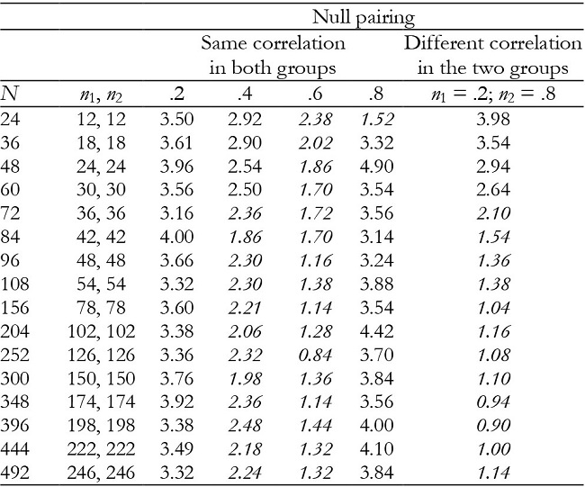
Table 1: Empirical Type I error rates (in percentages) for the group effect in balanced groups with K = 2.
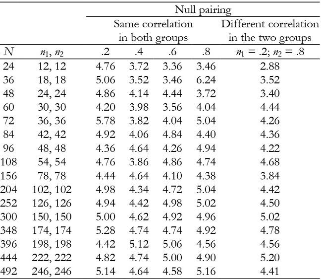
Table 2: Empirical Type I error rates (in percentages) for the time effect in balanced groups with K = 2.
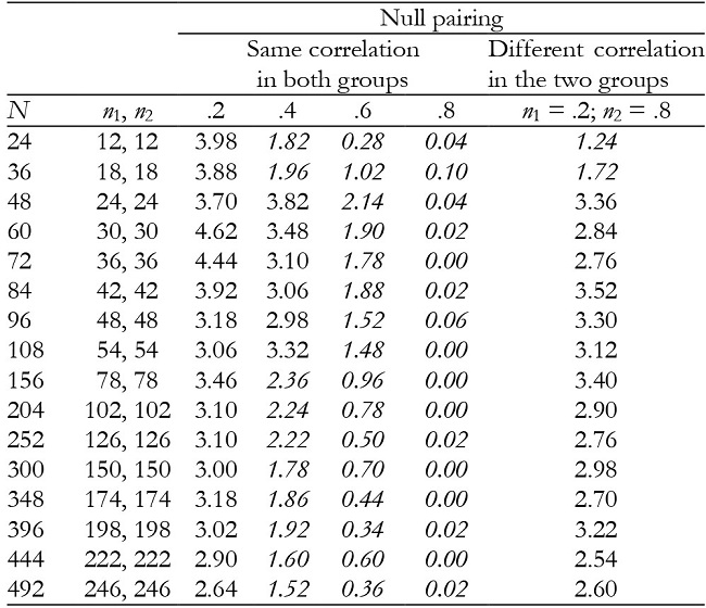
Note:In italics = conservative.
Table 3: Empirical Type I error rates (in percentages) for the interaction effect in balanced groups with K = 2.
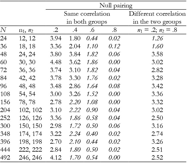
Note:In italics = conservative.
Table 4: Empirical Type I error rates (in percentages) for the group effect in balanced groups with K = 3.
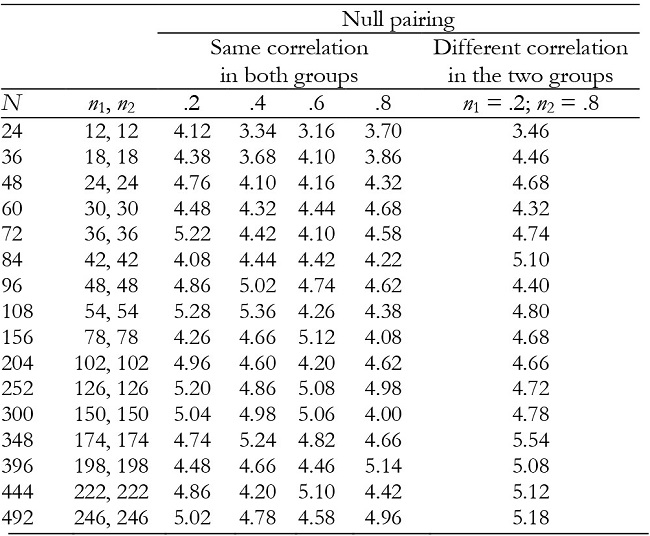
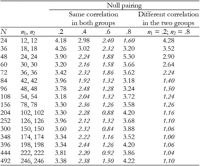
Table 5: Empirical Type I error rates (in percentages) for the time effect in balanced groups with K = 3.
Note:In italics = conservative.
Table 6: Empirical Type I error rates (in percentages) for the interaction effect in balanced groups with K = 3.
Note:In italics = conservative.
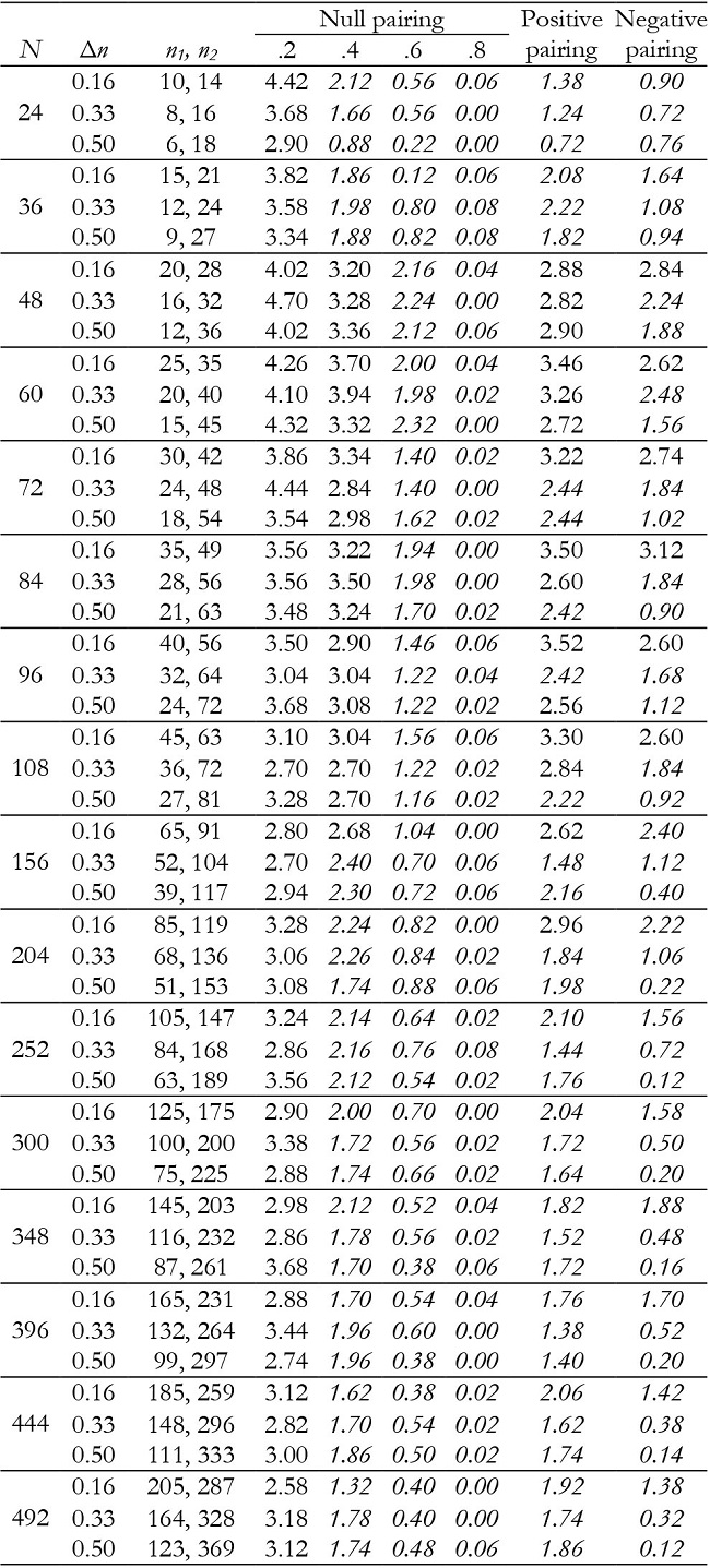
Table 7: Empirical Type I error rates (in percentages) for the group effect in unbalanced groups with K = 2.
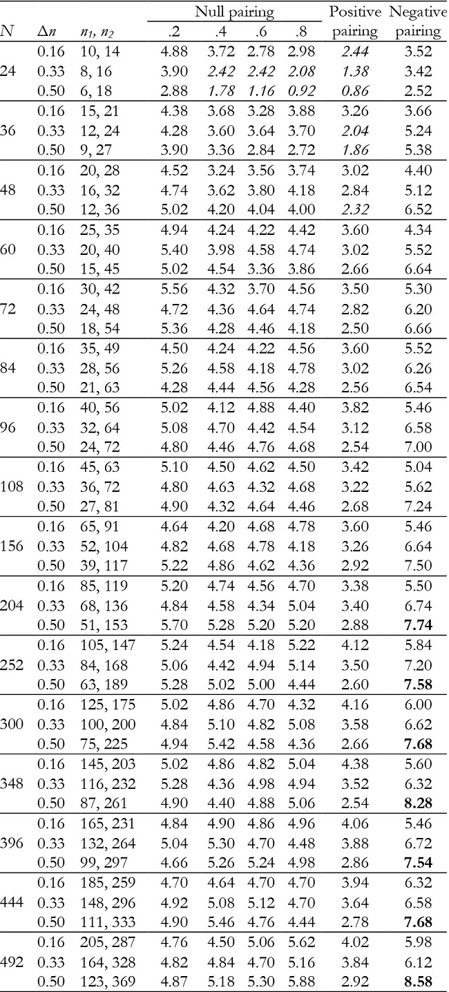
Note:Δn = coefficient of group size variation; null pairing: same correlation in the two groups; positive pairing: correlation .2 for n1 and correlation .8 for n2; negative pairing: correlation .8 for n1 and correlation .2 for n2; in ital-ics = conservative; in bold = liberal.
Table 8: Empirical Type I error rates (in percentages) for the time effect in unbalanced groups with K = 2.
Note:Δn = coefficient of group size variation; null pairing: same correlation in the two groups; positive pairing: correlation .2 for n1 and correlation .8 for n2; negative pairing: correlation .8 for n1 and correlation .2 for n2; in italics = conservative.
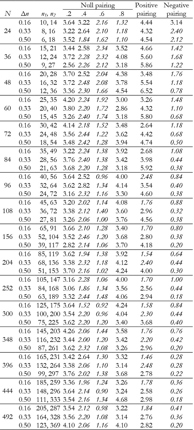
Table 9: Empirical Type I error rates (in percentages) for the interaction effect in unbalanced groups with K = 2.
Note:Δn = coefficient of group size variation; null pairing: same correlation in the two groups; positive pairing: correlation .2 for n1 and correlation .8 for n2; negative pairing: correlation .8 for n1 and correlation .2 for n2; in ital-ics = conservative.
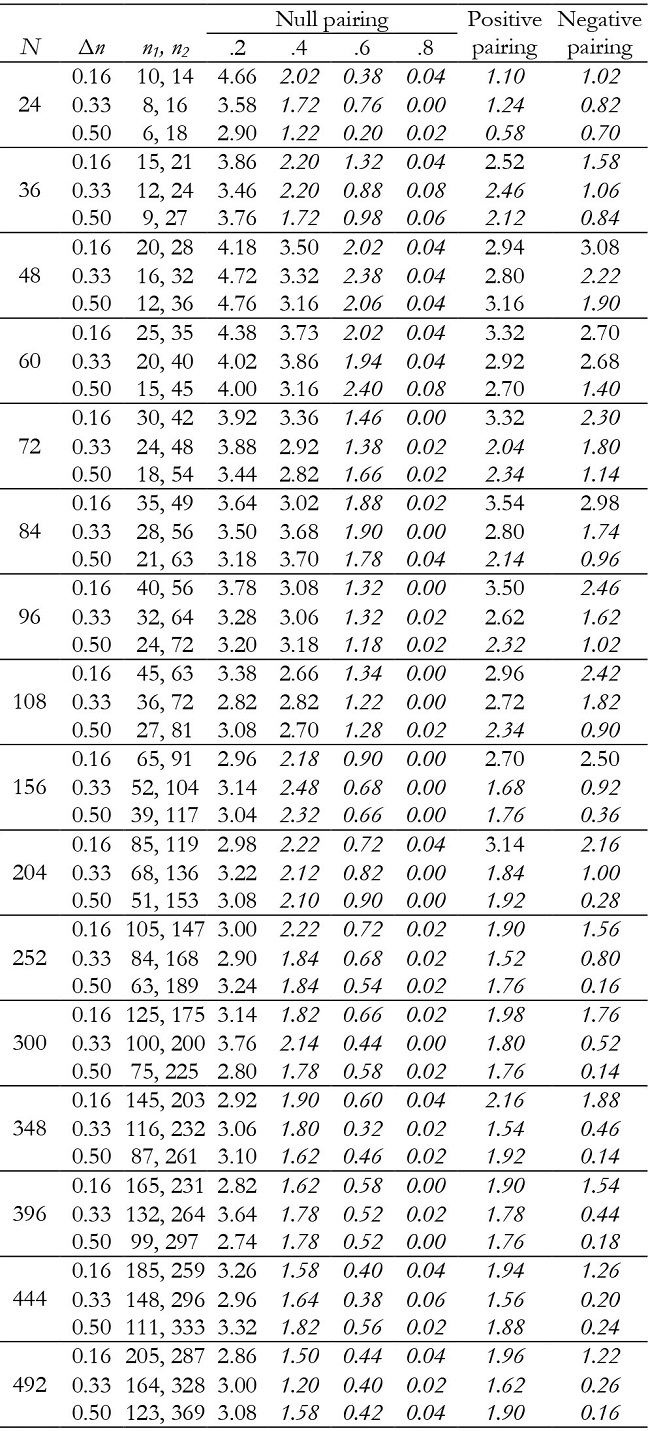
Table 10: Empirical Type I error rates (in percentages) for the group effect in unbalanced groups with K = 3.
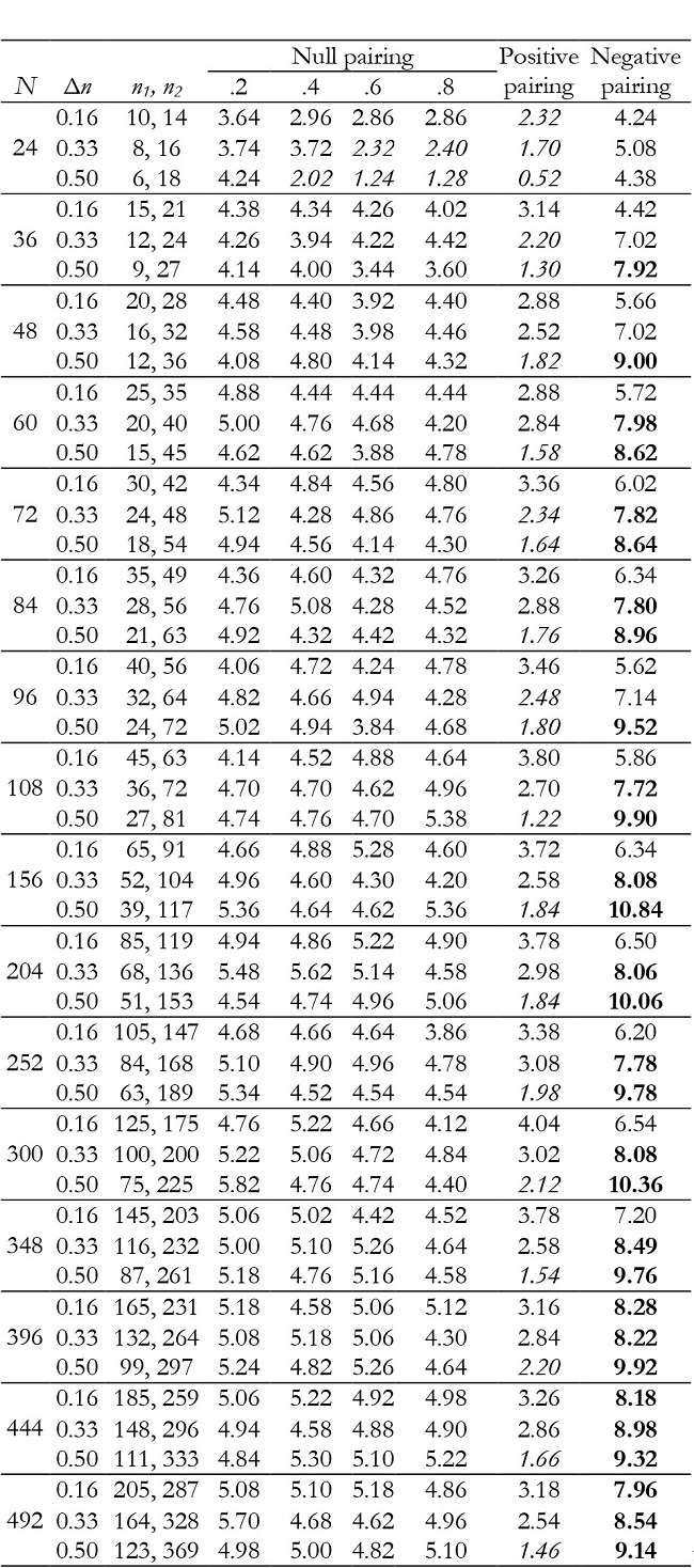
Note:Δn = coefficient of group size variation; null pairing: same correlation in the two groups; positive pairing: correlation .2 for n1 and correlation .8 for n2; negative pairing: correlation .8 for n1 and correlation .2 for n2; in ital-ics = conservative; in bold = liberal.
Table 11: Empirical Type I error rates (in percentages) for the time effect in unbalanced groups with K = 3.
Note:Δn = coefficient of group size variation; null pairing: same correlation in the two groups; positive pairing: correlation .2 for n1 and correlation .8 for n2; negative pairing: correlation .8 for n1 and correlation .2 for n2; in ital-ics = conservative; in bold = liberal.
Table 12: Empirical Type I error rates (in percentages) for the interaction effect in unbalanced groups with K = 3.

Note:Δn = coefficient of group size variation; null pairing: same correlation in the two groups; positive pairing: correlation .2 for n1 and correlation .8 for n2; negative pairing: correlation .8 for n1 and correlation .2 for n2; in ital-ics = conservative.
Five thousand replications of each combination of the above variables were performed at a significance level of .05.
Once the data had been generated, the GLMM was applied using proc glimmix. The classification variables were subject, group, and time. The fixed effects of the model were group, time, and interaction (group x time). The RSPL approach was used because its focus is the individual response. A binomial distribution was fitted with the logit link function, which is widely used for binary responses (Malik et al., 2020). For the adjustment of degrees of freedom, we used the Kenward-Roger approximation (Kenward & Roger, 2009), specifically the improved (KR2) method in SAS. This approach uses a less biased precision estimator and is recommended when analyzing repeated measures data (Stroup et al., 2018). This correction further reduces the precision estimator bias for the fixed and random effects under nonlinear covariance structures. Finally, the random effects were intercept and the slope over time. For the time variable, the AR(1) covariance structure was fitted. This correlation structure is close to an autoregressive structure, which is usually expected in repeated measures data (Gawarammana & Sooriyarachchi, 2017; Dang et al., 2008; Liu et al., 2012).
Data analysis
Robustness was evaluated by means of Bradley’s (1978) criterion, according to which a test is considered robust when the empirical Type I error rate is between .025 and .075 for a nominal alpha level of .05. When the empirical Type I error rate is above the upper limit, the test is considered liberal, and when it is below the lower limit it is considered conservative. The effects of the group factor, time factor, and interaction factor (group x time) were analyzed for each combination of manipulated variables.
Results
Balanced groups
In balanced groups, with K = 2 and K = 3, the group effect was robust in all conditions (Tables 1 and 4), including when the groups had different correlation values between repeated measures (null pairing between correlation and group size).
For K = 2, time and interaction effects were robust with correlation of .2, but the results became increasingly conservative as the correlation increased (Tables 2 and 3). They were also generally robust with null pairing.
For K = 3, time and interaction effects were robust with correlation of .2 and .8, while with correlation of .4 and .6 the results were conservative in the majority of conditions (Tables 5 and 6). They were also conservative with null pairing between correlation and group size in the majority of conditions.
Unbalanced groups
In unbalanced groups, for K = 2 and null pairing the group effect was robust in almost all conditions (Table 7), except with a small sample size (N = 24), where it can become conservative. For positive pairing between group size and correlation the test tended to be conservative with small sample sizes, whereas for negative pairing it tended to be liberal when inequality of group sample size was high in moderate and large sample sizes. For K = 3, it was conservative with positive pairing and liberal for negative pairing (Table 10).
For K = 2, time and interaction effects were robust with correlation of .2. However, the effects were increasingly conservative as the correlation increased (Tables 8 and 9), especially with correlation of .6 and .8. They were also conservative with both positive and negative pairing between group size and correlation.
For K = 3, time and interaction effects were robust with correlation .2 and .8, although with correlation of .8 and very small samples they were conservative. Results were generally conservative with correlation of .4 and .6 (Tables 11 and 12). They also tended to be conservative for positive pairing between group size and correlation as the sample size increased (from N = 96), and for negative pairing in all conditions.
Discussion
The aim of this study was to examine the empirical Type I error rates associated with the use of GLMMs under the most common conditions found in research in psychology (sample sizes less than 500, two groups, two and three repeated measures, and binary data). The RSPL approach in proc glimmix was used because its focus is on individual responses. In view of the fact that longitudinal data are normally correlated, the AR(1) covariance structure was fitted, and because the simulated samples were smaller than 500 we used the improved Kenward-Roger approach.
The results of this study provide researchers with useful information about the performance of these models, especially under extreme conditions (e.g., small samples, unbalanced groups, different correlation between repeated measures in each group). The most important conclusions in split-plot designs are:
For the group effect and balanced groups, the GLMM was always robust, including when the correlation between repeated measures of each group was different.
For the group effect and unbalanced groups, the GLMM can be (a) conservative when pairing between group size and the correlation between repeated measures is positive, and (b) liberal when this pairing is negative. With negative pairing the test became systematically more liberal as the inequality of group sample size increased.
-
For the time and interaction effects, the empirical Type I error rates of the GLMM depend on the correlation between repeated measures, the pairing between group size and correlation, the inequality of group sample sizes, and the number of repeated measures. Specifically:
The GLMM was robust with low correlation between repeated measures (.2) for all conditions studied.
When correlations between repeated measures were equal in the groups, the GLMM was generally conservative for medium values of correlations (.4 and .6). However, for high values (.8) it was only conservative with two repeated measures.
When correlations between repeated measures were different in the groups, the GLMM was generally conservative for both positive and negative pairing in unbalanced designs. It was also conservative for three repeated measures and null pairing in balanced designs.
As the inequality of group sample sizes increased, the GLMM was systematically more conservative for negative pairing.
For time and interaction effects, the GLMM analyzed in this study is generally robust with low correlation between repeated measures. However, with medium correlation it tends to be conservative, and researchers would therefore need to exercise caution before accepting the null hypothesis based on their results. We also found that the test is robust with K = 3 when the correlation between measures is .8. It is also important to note that for the group effect the test may become very liberal in the case of negative pairing between group size and correlation, and hence any significant differences between groups would need to be interpreted with care.
Dang et al. (2008) found that robustness of the GLMM in terms of power estimates depends on the within-subject correlation of the binary outcomes. Specifically, if the random effects remain the same but the within-subject correlations increase, the estimated power decreases. Although other simulation studies have examined the robustness of the GLMM with binary responses (e.g., Fang & Louchin, 2013; Gawarammana & Sooriyarachchi, 2017), their results cannot be compared with our findings here as the variables manipulated and study objectives were different.
Gawarammana and Sooriyarachchi (2017) showed that with three repeated measures, a binary response variable, the logit link function, and quadrature estimation, proc glimmix yielded satisfactory results with respect to Type I error for sample sizes above 20. Here we used proc glimmix in SAS, although other options with binary data are proc nlmixed, which is useful for nonlinear mixed models (Zhang et al., 2011), and proc genmod, which is useful for generalized estimating equations (Gawarammana & Sooriyarachchi, 2017; Landerman et al., 2011). Zhang et al. (2012) analyzed the use of proc nlmixed with binary data, obtaining robust results under correct model assumptions and with a relatively small number of random effects. Gawarammana and Sooriyarachchi (2017) concluded that proc genmod only works well when the sample size is very large (250 or over). In the review by Bono et al. (2021), none of the empirical studies they analyzed reported using proc nlmixed or proc genmod, and hence they did not compare the two procedures. It should be noted nonetheless that when applied to the modeling of binary responses, different procedures within a package may give quite different results (Zhang et al., 2011).
The robustness of the GLMM also differs depending on the parameter estimation method used (Zhang et al., 2012). Here we only used the RSPL, as this is well suited to the objectives of research in psychology. It is important to note, however, that empirical studies in the field of psychology that are based on the GLMM rarely report the estimation method used (Bono et al., 2021). Furthermore, few studies focused on the GLMM have examined methods of correcting the degrees of freedom for small samples (Bell & Grunwald, 2011). Li and Redden (2015) compared the Kenward-Roger procedure with other methods of adjusting the degrees of freedom when the GLMM is used to analyze binary outcomes in small sample cluster-randomized trials. They found that the Kenward-Roger method can provide tests with very conservative Type I error rates.
Many of the results derived from simulation studies may be of little use to applied researchers in the psychological field, because the manipulated variables and their values (e.g., sample size, number of groups, number of repeated measures, correlation, etc.) show considerable heterogeneity and are rarely chosen based on research practice. Hence our aim in this simulation study was to provide empirical evidence about the robustness (in terms of Type I error) of the GLMM in split-plot designs with binary response variables. To achieve this aim, we systematically manipulated a broad set of variables and range of values, based on research practice in psychology and related fields.
Our focus here has been on the analysis of repeated binary data. However, the GLMM can be considered for other types of outcomes, such as repeated ordinal responses (Lin, 2010; Lin & Chen, 2016) or repeated count measures (Bell & Grunwald, 2011; Huang et al., 2016; Zhang et al., 2012). Other important issues related to the performance of GLMMs that are not discussed in this paper are the approach chosen to deal with missing data or attrition (Amatya & Bhaumik, 2018; Miller et al., 2020; Noh et al., 2012), overdispersion (Johnson et al., 2015), misspecification of the shape of a random effects distribution (Litière et al, 2007; McCulloch & Neuhaus, 2011), link function misspecification (Yu & Huang, 2019), and the impact of different random effects covariance matrices for longitudinal data (Hoque & Torabi, 2018). Although much more research is still required in this area, the results obtained in the present study provide useful information about the performance of GLMMs in psychological research settings. This is important as applied researchers can now use statistical software and specific packages (e.g. SAS, R, and SPSS) to conduct GLMM analyses.
It should be noted that although we simulated a broad set of variables and range of values, the conclusions to be drawn are limited by the range of evaluated conditions. For example, we studied only one model for binary outcomes, and we did not evaluate model performance with alternative link functions or estimation methods. These limitations are potentially fruitful directions for future research. Finally, the robustness of the GLMM can also be studied in terms of power (Chen et al., 2016; Stroup, 2013). Despite the increasing use of GLMMs, there are few articles reporting a power analysis for these models (e.g., Dang et al., 2008; Jiang & Oleson, 2011; Johnson et al., 2015; Kain et al., 2015). A further study analyzing the robustness of the GLMM in terms of power and calculating the optimal sample, as proposed for the LMM (Vallejo et al., 2019), would therefore provide a useful complement to the present results.

