An ecological study of Hungarian suicide data using complex statistical methods

 

 

Zoltán Kmetty^a; Károly Bozsonyi^b and Tamás Zonda^c

^a ELTE Faulty of Social Studies, Sociological Institute, Budapest. Hungary
^b Károli Gáspár University of the Reformed Church in Hungary, Institute of Social and Communication Sciences, Department of Communication, Budapest. Hungary
^c Hungarian Association for Suicide Prevention. Hungary

Correspondence

 

 

---

ABSTRACT

Background and Objectives: According to a number of psychiatrists, the decrease in the number of suicides can almost exclusively be ascribed to the increasing use of new antidepressants (ADs). Several ecological studies have been carried out to lend support to this claim; unfortunately, many of these started out from either methodologically or statistically flawed assumptions. The purpose of the current study is to demonstrate the examined relationships using complex time-series techniques on Hungarian national sample.
Methods: When investigating the relationships between our time series, first we ensured their stationarity using several methods. We used two methods for the analysis involving several independent variables.
Results When using dynamic regression to ensure stationarity, the residuals of the suicide and AD time series showed a significant negative correlation. At the same time, when using the more robust technique of time series differentiation, the stationary time series showed no significant relationship between the use of antidepressants and suicide rates.
Conclusions The models fitting our data showed somewhat mixed results. The vagueness of ecological models is well demonstrated by the fact that even those sociological variables (number of divorces, alcohol consumption) failed to show a significant relationship with suicides here, which are usually significant in analyses using micro data.

Keywords: Suicide rate; Use of antidepressants; Ecological study; Complex methodology.

---

 

Introduction

In the middle of the 1980s, the number of suicides started to decrease in most countries of Europe, and so did the number of deaths caused by several harmful phenomena (such as fatal accidents, smoking, alcoholism) and several illnesses (cardio- and cerebral-vascular). The economic boom and the resulting improvement in the overall quality of healthcare are probably not negligible factors in this¹.

According to a number of psychiatrists, the decrease in the number of suicides can almost exclusively be explained by the increase in the sales (and usage) of new antidepressants (AD). Researchers investigating the topic have attempted to find support for this relationship using ecological studies. The results of ecological studies project a mixed picture; although at the moment studies suggesting a relationship between the increasing use of antidepressants and the decrease in the number of suicides on the level of the whole population are in majority², but there are also a number of counterexamples³.

Several pieces of criticism can be raised against ecological studies both on theoretical and methodological grounds. On the one hand, it is clear that ecological analyses can only detect relationships between two phenomena, but they cannot establish causality; methodologies applying controlled experimental designs would be needed for that⁴. Obviously, this dilemma is valid for all conclusions that are not based on an experimental setup. On the other hand, there is a possibility that because of the use of aggregate data, we fall victim to false ecological conclusions⁵. This practically means that the relationship between certain variables can even be opposite in direction at the individual and aggregate levels, as shown by several examples in the literature. The possibility of ecological fallacy fundamentally reduces the validity of the conclusions that can be drawn based on these models^6,7.

Besides these important theoretical dilemmas, the ecological models based on time series reflecting changes in suicide rates struggle with further methodological problems. We would like to highlight two of these which have not attracted much attention either in the Hungarian or in the international literature.

A survey of the literature sheds light on the fact that a vast majority of studies disregard that time series observations are usually statistically not independent of one another in time, which often leads to the use of inappropriate statistical tools. In the case of time series, showing the similarity of curves is not enough, just like simple correlational or linear regression models are also inadequate in themselves because the widely used standard models of these methods require the independence of observations. The assumption of independence is violated in this case because values of the given period depend on those of the previous period (or even on those of other preceding periods). In time series analysis, this is called the problem of autoregressivity. A given time series can be affected by several components, such as trend, seasonal or cyclical components, which can be interpreted in time. [Moreover, analysing autoregression and/or moving average processes (ARIMA) is also quite common in the case of time series.] Models of causal relationships between time series often assume the stationarity of time series. Time series containing trend-cycle and/or periodic components cannot be considered stationary. Besides non-stationarity, autoregressivity can also be held responsible for the fact that standard correlational and similar statistical methods can easily lead to erroneous results^8-11.

The statistical rigour applied in this study is deliberate; faulty model specifications are quite frequent even in articles that are often cited in the literature.

In their frequently cited study, Ludwig, Marcotte and Norberg¹² employ an impressive battery of statistical tools to support the relationship between data on suicide and antidepressant use. The R² fit indices that are over 95% percent in their study seem to suggest, however, that the models they applied are probably considerably overfitted (although we cannot be certain of this, as, in defiance of academic standards of publication, they fail to provide the degrees of freedom of their models). These extremely high R² indices are outstanding even in the case of ecological models. But they fail to report the degree of freedom of the models, similarly to the extent of multicollinearity between the variables. Entering the time "variable" into the model helps with stationarity (although it does not solve it completely), but based on data trends, it also introduces a large degree of multicollinearity into the models, which leads to the overestimation of standard errors, and thus, a misjudgement of significance.

Among more recent studies, the paper of Gusmao and colleagues¹³ received considerable attention. At the beginning of their paper, they analyse the raw relationships between suicide time series and antidepressant use with the help of correlational methods; problems involved in this have already been pointed out above. They use more complex models in the second part of their paper, which at first sight seem to result in convincing findings concerning the use of antidepressants. Nevertheless, the authors themselves admit that they had to leave the time component out of the analysis, as it annulled all other relationships including the effect of ADs that they intended to support. Moreover, they fail to report measures of fit for all models; therefore, it does not come to light whether it is multicollinearity caused by a presumably very strong positive correlation between GDP and antidepressant use that can be held responsible for problems of fit.

Statistical dilemmas discussed so far basically derived from problems of stationarity, but we neglected another important issue, the length of time series. On the one hand, in the case of any two time series with deterministic trends, the size of correlation between them is basically determined by the length of the time series exclusively. If we have two time series with the same monotony (increasing-increasing or decreasing-decreasing), then the threshold limit of the correlation between the two time series approaches +1 with the increase in time. The length of time series, that is the number of cases, does not only decrease the standard error of measurement, but the validity of the estimate also weakens. In these cases, our statistical estimates are biased, and therefore, not valid. This problem can be handled by making our time series stationary. The issue of the shortness of time series is rarely raised in the literature although it is also a quite common phenomenon. In the case of time series analysis, a certain number of cases are required for drawing reliable conclusions. There are no strict rules about this, but the limit is usually set at 30 observations, which can also be a much greater number if we would also like to fit seasonal components in the model. In the case of short periods, further analyses are required in order to arrive at reliable results.

 

Methods and data

In the introductory section, we presented a quite detailed overview of the theoretical and statistical problems posed by ecological models. Although we cannot provide satisfactory solutions for issues of causality and ecological misinterpretation, the independence of time series can be assured using complex models. We are going to present such complex statistical analyses in the following sections using Hungarian data.

In our analysis, we investigated the relationships between the suicide rate (number of suicides per 100 thousand residents) (Hungarian Statistical Office database) and the sales of antidepressants (NO6AA^§, NO6AB^§§, NO6AG^§§§, NO6AX^§§§§ in pharmacies and hospitals in total, in the format suggested by WHO, i.e. DDD/1000 residents/day) between 1982 and 2011 at the national level (OEP and IMS database)^§§§§§. We included several background variables in our analysis, such as the GDP (in comparison to the base year of 1960), the number of divorces per 1000 residents, the number unemployed per 100 residents, and the absolute alcohol consumption per capita. The source of these variables was the database of the Hungarian Central Statistical Office; however, figures of unemployment were only available for the period after 1998. All the raw data were presented in the Appendix table A1. Official, ethical approval was not requested in view of the nature of this study.

 

 

The statistical program package R¹⁴ was used for data analysis; besides the basic packages, commands of the tseries¹⁵, the MSBVAR¹⁶ and the forecast¹⁷ packages have been used.

The stationarity of the examined time series

As we have argued above, a precondition of using most analytical tools (e.g. correlations) in the case of time series analysis is that both time series should be stationary. Therefore, before applying correlational analyses, it has to be established whether the assumption of stationarity is satisfied. We examined this using both graphic and statistical tests. Figure 1 presents the autocorrelation function plots (from now on referred to as ACF) of suicide rates and AD consumption time series. The ACF shows the correlations between the time series at various time lags for the given time series.

 

 

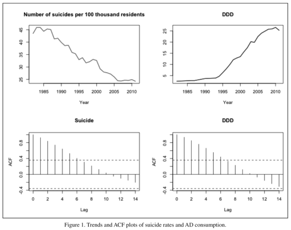
On the left hand side of Figure 1, the ACF plot of the suicide time series, while on the right hand side of Figure 1, the ACF plot of the AD consumption time series can be seen. It is quite obvious in the case of both plots that correlation with time lag 1 is very high, which means that the value for the given year is greatly determined by value of the previous year. These figures already suggest that these time series are non-stationary although statistical tests are also needed to ascertain this. In our analysis, we used two well-known and acknowledged statistical tests¹⁸ for these purposes. The Augmented Dickey-Fuller test (ADF) is one of the most frequently used methods for establishing stationarity¹⁹. The basis of the test is the following regression model, y′_t = Φy_t-1 + β₁ y′_t-1 + β₂ y′_t-2 + ... + β_k y′_t-k, where y′_t = y_t - y_t-1 is the first differential of the time series, and k is the number of differentials. If the original time series has to be differentiated in order to make it stationary, then phi has to be less than 0. The null hypothesis of the ADF test is that the given time series is non-stationary.

The other procedure is the KPSS (Kwiatkowski-Phillips-Schmidt-Shin) test²⁰. The null hypothesis here is the opposite of the above, that is, the time series is supposed to be stationary. Results of these tests for the variables investigated are presented in Table 1.

 

 

ADF tests recommend that if p > 0.05 then the null hypothesis should be kept, which means that the time series are non-stationary. This is also confirmed by the results of the KPSS tests (where p < 0.05 means that the time series are non-stationary). (The only exception here is the time series of the divorces.) The results of the tests clearly show that as a first step of the analysis, the time series need to be made stationary before any further calculations can be carried out.

First method

There are several methods of making a time series stationary. Time series with any identifiable trends are definitely non-stationary. Therefore, by "removing" the trend from the time series, the probability of stationarity increases. "Filtering" the trend, however, is not necessarily sufficient to make the time series stationary; the residual might still be autocorrelated. In case the residual is autocorrelated, it might be worth examining whether autoregressive or moving average processes (ARIMA) can be identified in the time series. There is an established procedure for the joint modelling of trend and ARIMA processes; it is called dynamic regression⁹. The procedure involves including all our variables in a dynamic regression model, which contains one trend parameter and if necessary the ARIMA process to ensure that the residual is not autocorrelated. In practice, the correlation analysis of the regression residuals comprises the first method of investigation.

Table 2 summarises the regression coefficients of the trends for each variable, and whenever it was required the type of ARIMA process identified.

 

 

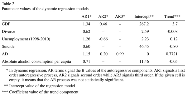
After fitting the above regression models, the residuals were stationary; therefore, it was possible to search for relationships between them using correlations and other techniques. Results of Table 2 indicate that no moving average processes are identifiable in the case of any of the variables; however, AR processes can be found in each case. In the case of antidepressant use this involves AR1, AR2 and AR3, which suggests that in statistical models, it is not necessarily enough to filter for the AR1 process only.

Second method

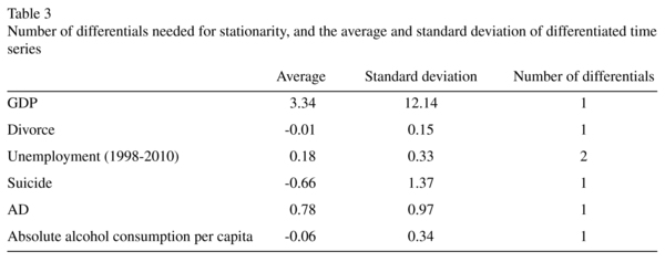
In the case of non-stationary time series, the differentiation of time series is also a standard procedure. The first-order differential shows the change in comparison with the t-1 time slot of the time series. In the case of suicides, the first-order differential shows the change in the yearly rate of suicides. The second examination technique is the investigation of the relationships between the differentiated time series using correlations. The following table (Table 3) presents the basic distributions of our differentiated variables, and it also shows the number of differentiations that were necessary for reaching stationarity (The first-order differential will not necessarily be stationary; therefore, the execution of further differentiations might be needed).

 

 

The second examination technique was the investigation of the relationships between the differentiated time series presented here, using correlations. Since the time series have become stationary as a result of differentiation, there can be no statistical objection to the use of correlations.

 

Results

Results of the first type of investigation

The first analytical scheme involved calculating the correlation coefficients between the residuals of the dynamic regression. The residuals of the suicide time series have been correlated with the residuals of the AD, GDP, unemployment, divorce and the absolute alcohol consumption time series (see Table 4).

 

 

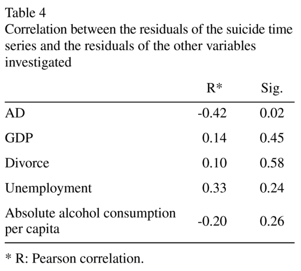
There is negative correlation between the residuals of AD and suicide time series at 5% significance level, but the relationship is statistically not significant at 1% level. The strength of the correlation is difficult to estimate primarily because of the low number of cases; it is within the -0.08 to -0.68 range at 95% confidence level. The relationships were statistically not significant in the case of the other four variables.

Besides pair-wise correlations, a regression model has been fitted to the residuals of the suicide time series. From the independent variables, the number of unemployed was not entered into the model, as there was no data available for the whole of the time series. As it could be expected on the basis of the correlation tables, the data could not be fitted into a significant regression model (p = 0.06).

Results of the second type of investigation

The second method applied was the correlational analysis of differentiated time series. Using the differentials of the time series is a more robust method than the dynamic regression presented in the first analytical scheme; therefore, in this case the reliability of the results is higher. The next Table (Table 5) presents the relationships between the differentiated suicide time series and the other variables involved in the analysis.

 

 

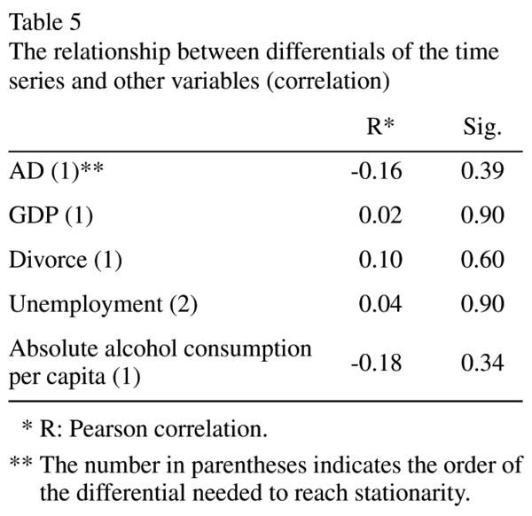
None of the five possible background variables examined by us showed a relationship with the suicide time series. Therefore, the correlation between AD and suicides identified in the case of the residual time series was not supported by the analysis of differentiated time series. Fitting of a regression model was also attempted for the differentiated time series, but it was not possible here either (p = 0.65).

Granger-Cause

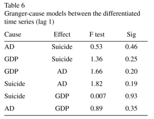
A third method was also applied for testing the relationships. Although, as we stated before, in the case of ecological models establishing causal relationships is not possible, there are certain statistical constellations which might signal causal relationships; such an important constellation is the Granger-cause²¹. In the case of time series, X time series is regarded as the Granger-cause of Y time series if the past values of X help in predicting Y. When attempting to identify the Granger-cause in the case of stationary time series, we attempt to fit such a regression model in which past values of X, the value of X, as well as past values of Y are used to estimate Y. The magnitude of the "lag" parameter heavily depends on the length of the time series, and similarly to general regression models, overfitting has to be avoided. Since the length of our time series was only 30 years (and 29 for the differentiated time series), only the X and Y values of the t-1 time slot were included in the regression model.

Results showed (see Tables 6 and 7) that neither ADs nor the GDP is the Granger-cause of the rate of suicides either based on the residuals of dynamic regression or based on differentiated time series. The model that is closest to reaching statistical significance in one where suicide is presented as a cause and antidepressant consumption as a result. It is important to note that based on the model, no relationship can be established between the GDP and AD consumption either.

 

 

 

Discussion

When analysing the Hungarian data, we aimed to examine the relationship between AD consumption (usage) and suicide rates, emphasising that ecological analysis does not establish causal relationships. Nevertheless, it is possible and rather important to examine the statistical co-occurrence of certain variables. When examining relationships between time series, the stationarity of our time series needs to be ensured as the first step before the analysis of any possible relationships between them. We applied two methods for this. On the one hand, based on the dynamic regression procedure, trend and ARIMA effects were partialled out of the models. The thus calculated residuals of the suicide and AD time series displayed a negative relationship at the national level.

We also attempted to make the time series stationary by differentiation. The differentiated time series calculated with the help of this more robust method showed no relationshipbetween the use of antidepressants and suicide rates at the national level. An important aspect of our results is that those regression models where the relationship between AD and suicide was investigated while controlling for several variables at the same time were statistically not significant. The latter results are further supported by the fact that the rate of suicide was not Granger-caused by the quantity of antidepressants sold.

These relationships were also investigated at the level of counties using the methods presented in this paper, and no significant relationships were found in any of the cases. In the case of county level time series, we only had 10 years of data available; therefore, the low statistical strength might have also been caused by the shortness of time series.

We would like to emphasise that our results do not mean that there is no relationship between AD and suicides, but they indicate that, for the period between 1982 and 2011, it is impossible to identify clear-cut relationships between the variables examined. Therefore, the strong negative statistical relationship supported by econometric models presented in the literature should be treated with caution. In contrast with that we have to take in mind that our models haven't included indicators measuring the global improvement in the resources of mental health care or changes in the patterns of prescription of antidepressants. In the other hand it is also an important finding that based on the models presented in this paper, there is no ecological relationship between suicide, the GDP, divorce, the number of unemployed or alcohol consumption either. The fact that background variables which otherwise seem "to work" are not significant in ecological models shows that results which can be obtained from these models should be treated with caution in general.

 

Declaration of interest

The authors report no conflicts of interests. The authors alone are responsible for the content and writing of the paper.

 

---

§ Non-selective monoamine reuptake inhibitors.

§§ Selective serotonin reuptake inhibitors.

§§§ Monoamine oxidase A inhibitors.

§§§§ Other antidepressants like Oxitriptan, Tryptophan, Mianserin etc.

§§§§§ As this is an ecological study we haven't used any micro data, only aggregated data on yearly bases. In this form the anonymity of cases are granted by the research design. For the analysing of this data structure no approval of the Institutional Review Board is needed.

 

References

1. European health for all database (HFA-DB) WHO Regional Office for Europe (Updated: Apr. 2014).         [ Links ]

2. Milner A, McClure R, De Leo D. Socio-economic determinants of suicide: an ecological analysis of 35 countries. Soc Psychiatry Psychiatr Epidemiol. 2012; 47(1): 19-27.         [ Links ]

3. Titelman D, Oskarsson H, Wahlbeck K, Nordentoft M, Mehlum L, Jiang GX, et al. Suicide mortality trends in the Nordic countries 1980-2009. Nord J Psychiatry. 2013; 67(6): 414-23.         [ Links ]

4. Imai K, Keele L, Tingley D, Yamamoto T. Unpacking the Black Box of Causality. Learning about Causal Mechanism from Expreminental and Observational Studies. American Political Science Review 2011, 105(4): 765-89.         [ Links ]

5. Robinson WS. Ecological Correlations and the Behavior of Individuals. American Sociological Review. 1950, 15(3): 351-7.         [ Links ]

6. Piantadosi S, Byar DP, Green SB. The ecological fallacy. Am J of Epidemol. 1988 127(5): 893-904.         [ Links ]

7. Schwartz S. The fallacy of the ecological fallacy: the potential misuse of a concept and the consequences. Am J Public Health 1994. 84(5): 819-24.         [ Links ]

8. Bramness JG, Walby F. Ecological studies and the big puzzle of falling suicide rates. (Editorial) Acta Psychiatr Scand. 2009; 119:169-70.         [ Links ]

9. Wakefield J. Ecologic studies revisited. Annu Rev Public Health 2008; 29:75-90.         [ Links ]

10. Default B, Klar N. The Quality of Modern Cross-Sectional Ecologic Studies: A Bibliometric Review. Am J Epidemiol. 2011; 174(10): 1101-7.         [ Links ]

11. King G. A Solution Inference Problem. Princeton Univ. Press. 2013.         [ Links ]

12. Ludwig J, Marcotte DE, Norberg K. Anti-depressant and Suicide. J Health Econ. 2009; 28(3): 659-76.         [ Links ]

13. Gusmão R, Quintão S, McDaid D, Arensman E, Van Audenhove C, Coffey C, et al. Antidepressant Utilization and Suicide in Europe: An Ecological Multi-National Study. PLoS One. 2013; 8(6): e66455.         [ Links ]

14. R Core Team (2012). R: A language and environment for statistical computing. R Foundation for Statistical Computing, Vienna, Austria. ISBN 3-900051-07-0, URL http://www.R-project.org/.         [ Links ]

15. Trapletti A, Hornik K. Time Series Analysis and Computational Finance. R package version 0.10-32. 2013. http://cran.r-project.org/web/packages/tseries/tseries.pdf.         [ Links ]

16. Brandt P, Markov-Switching. Bayesian, Vector Autoregression Models, R package version 0.9-1. 2014. http://cran.uvigo.es/web/packages/MSBVAR/MSBVAR.pdf.         [ Links ]

17. Hyndman R, Khandakar Y. Automatic time series forecasting: The forecast package for R. Journal of Statistical Software 2008; 26 (3). http://www.jstatsoft.org/v27/i03/paper.         [ Links ]

18. Hyndman R, Athanasopoulos G: Forecasting: principles and practice. Otext https://www.otexts.org/fpp/ (Accessed: 2013).         [ Links ]

19. Banerjee A, Dolado JJ, Galbraith JW, Hendry DF. Cointegration, Error Correction, and the Econometric Analysis of Non-Stationary Data, Oxford University Press, Oxford. 1993.         [ Links ]

20. Kwiatkowski D, Phillips PCB, Schmidt P, Shin Y. Testing the null hypothesis of stationarity against the alternative of a unit root. Journal of Econometrics. 1992; 54 (1-3): 159-78.         [ Links ]

21. Granger CWJ. Investigating Causal Relations by Econometric Models and Cross-Spectral Methods. Econometrica 1969; 37: 424-38.         [ Links ]

 

 

Correspondence:
Kmetty Zoltán
1133 Budapest
Kárpát utca 16 V/19
Tel: +363 036 646 11
E-mail: zkmetty@tatk.elte.hu

Received: 6 March 2016
Revised: 27 July 2016
Accepted: 4 August 2016