


 Servicios personalizados
 Inglés (pdf)
 Articulo en XML
 Referencias del artículo
 Enviar articulo por email
 Citado por SciELO
  Citado por Google
  Similares en
SciELO
Similares en
SciELO  Similares en Google
 Permalink
The use of questionnaires or test to score individuals on a construct or latent variable is common in social and health sciences (test hereafter). Often, the test score is defined as the sum or the average of each person's responses to the test items and inferences about the construct must be based on sound psychometric properties of that score. Among other, evidence of test score reliability should be provided as stated in the standard 2.3 in Standards for Educational and Psychological Testing (American Educational Research Association [AERA] et al., 2014). One way to provide this evidence is to calculate internal consistency reliability, which is the focus of this paper.
The internal consistency reliability of a test score is based on the degree of association between the item responses obtained on a single administration of the test to a group of persons. The calculus is very simple in an idealised measurement model, in which all items assess a single construct (unidimensionality) with the same discriminating capacity (essentially tau-equivalent measures reflected in equal factor loadings). Moreover, measurement errors, considered present in all assessments, are random and unrelated (independent errors). On the other hand, the persons assessed conform a group with appreciable individual differences in the construct but homogeneous with respect to other characteristics. Non missing responses to a long test composed by homogeneously formatted items obtained from a big sample would bring this ideal scenario to completion.
In realistic settings, measurement models are more complex. Test items may measure different constructs (multidimensionality), or measure the same main construct, reflected in a general factor, with some of the items grouped into secondary factors or showing correlated errors (essential unidimensionality; e.g., due to similarly worded items or to items that, in addition to the main dimension, measure other minor dimensions). Moreover, items usually show different discrimination capacity (congeneric measures reflected in different factor loadings) and may show specific variance not shared with other items and not assimilable to measurement error (e.g., items evaluating different facets of a single construct). Furthermore, persons assessed may display other characteristics inducing heterogeneity or may even pertain to well-defined groups or classes. In front of any of these complexities, the ideal scenario described above is no longer realistic, not to talk about missing data, short test length or small sample size.
The best way to accommodate the estimation of reliability to realistic settings has been a matter of intense debate since the end of the last century. To set the debate, the following few paragraphs outline the basic concepts of measurement theory posited by three theories of measurement underpinning the calculation of an internal consistency coefficient
According to Classical Test Theory (CTT; Lord & Novick, 1968; see also Muñiz, 2018; Sijtsma & Pfadt, 2021), people's responses to the test items are expected to correctly reflect individual differences in the construct by producing variability in the scores. This between-person variability is the focus of the measurement and is referred to as systematic or true variance. The responses of individuals will also depend on many other minor factors present in the assessment, such as fatigue or motivation, which are considered to produce unpredictable variability referred to as error. If the item errors are independent of each other and independent of the true score, the total variance of the item sum or average is the sum of the systematic variance plus the error variance. Reliability coefficients are intended to quantify the proportion of systematic variance present in the total variance and therefore take values between 0 and 1, with high but not extreme values (not close to one) being preferable.
The most widely used estimate of internal consistency reliability is Cronbach's alpha coefficient (α), formulated by Cronbach (1951), among other authors, in the framework of CTT (Gulliksen, 1950) under the ideal scenario depicted above: unidimensional, essentially tau-equivalent measures with independent errors. Several equivalent formulas can be used to compute α, but in essence it is a ratio between the systematic variance and the total variance.
In the numerator, the average of covariances between items quantifies the systematic variance. In the denominator, the sum of elements of the variance-covariance matrix of items quantifies the total variance. When the total score is the item sum (or average) and data are close to the idealised scenario described above, the resulting ratio is a good estimate of the proportion of systematic variance present in the observed score variance.
Coefficient α is also a particular case of the intra-class correlation coefficients derived from the Generalizability Theory (GT; Cronbach et al., 1963, see also Brennan, 2001). The main objective of GT is to disentangle identifiable sources of error that contribute to the error variance in CTT. In this case, different measures of reliability are derived from random effects repeated measures ANOVA. Among the best known intra-class correlation coefficients, the consistency coefficient for average measures equals α. Based on covariation between repeated measures should not be confounded with the absolute agreement coefficient for average measures which includes the additional requirement of equal means between repeated measures.
In addition, internal consistency reliability can also be derived from Factor Analysis (FA; Thurstone, 1947; see also Brown, 2015; Ferrando et al., 2022). If the items measure a single factor with uncorrelated errors, item responses can be explained by a common part (or factor loading) plus a unique part (or uniqueness). Assuming standardised factor scores, McDonald (1999) defined the omega coefficient (ω) as the ratio between the common variance or the square of the sum of the factor loadings, and the total variance or the square of the sum of the factor loadings plus the sum of the uniquenesses. This coefficient has also been referred to as the composite reliability or reliability of a composite score (Raykov, 1997a), ωtotal (Revelle & Zinbarg, 2009) and ωu (Flora, 2020).
Finally, the FA and the CTT measurement models are equivalent when factor loadings are assimilated with the true variance and uniquenesses are assimilated with the error variance (e.g., Green & Yang, 2015). Then, α is a particular case of ω obtained in unidimensional data with uncorrelated errors and equal factor loadings for all items (essentially tau-equivalent measures). On the other hand, unidimensional data with uncorrelated errors and different factor loadings for some items (congeneric measures), will provide a value of α lower than that of ω. Both values, α and ω are equal to or lower than the population reliability, and thus both are lower bounds of reliability except for sampling variability. Because both coefficients are estimates based on samples, their values must be accompanied by confidence intervals (Oosterwijk, et al., 2019).
Finally, the FA and the CTT measurement models are equivalent when factor loadings are assimilated with the true variance and uniquenesses are assimilated with the error variance (e.g., Green & Yang, 2015). Then, α is a particular case of ω obtained in unidimensional data with uncorrelated errors and equal factor loadings for all items (essentially tau-equivalent measures). On the other hand, unidimensional data with uncorrelated errors and different factor loadings for some items (congeneric measures), will provide a value of α lower than that of ω. Both values, and ω are equal to or lower than the population reliability, and thus both are lower bounds of reliability except for sampling variability. Because both coefficients are estimates based on samples, their values must be accompanied by confidence intervals (Oosterwijk, et al., 2019).
At the end of the 20th century, α had no clear competence as an estimator of reliability, although misuses were already being reported (e.g., Cortina, 1993; Schmitt, 1996). From then on, a lively debate about the best estimator of internal consistency reliability has been growing. We will present the corners of the debate related to the methodological research, the publication habits of scientific journals, and the position of normative institutions.
In the first decade of the 21st century, a lot of methodological research was devoted to identifying and disseminating alternatives for α as better (lower-bound) reliability estimators. A first group of specialists advocated in favour of coefficients derived from FA such as ω (Green & Yang, 2009; Raykov, 1997a; Yang & Green, 2011), others argued in favour of coefficients not based on a specific measurement model, as the coefficient glb (greatest lower bound; Sijtsma, 2009), while a third group argued the use of several coefficients to express different aspects of internal consistency reliability (Bentler, 2009; Zinbarg et al., 2005). Later, the work of McNeish (2018) published in the journal Psychological Methods, advocated the use of several coefficients discouraging explicitly α. Meanwhile, simulation studies have shifted the debate from the best lower bound estimate to the most accurate estimate of the population reliability. No appreciable differences in accuracy between α and ω have been reported for a large number of measurement models (e.g., Edwards et al., 2021; Gu et al., 2013; Raykov & Marcoulides, 2015). Additionally, some coefficients not based on a measurement model have shown unacceptable behaviour when tested for accuracy in simulation studies (Edwards et al., 2021; Sijtsma & Pfadt, 2021). Lastly, the coefficient ω has been criticised due to the large number of intermediate decisions needed to obtain it (Davenport et al., 2016) and for the fact that ω does not refer to a single indicator but to a whole family of coefficients, which may difficult comparison between studies (Scherer & Teo, 2020; Viladrich et al., 2017). Based on some of these reasons, a growing number of voices is calling for a return to α, even coming from authors who had previously advocated other alternatives (Raykov et al., 2022; Sijtsma & Pfadt, 2021). Other positions consider that the use of α or other coefficients should depend on the fulfilment of their underlying assumptions (Green & Yang, 2015; Raykov & Marcoulides, 2016; Savalei & Reise, 2019; Viladrich et al., 2017). In addition, the joint publication of α and other alternative coefficient(s) has been proposed as a good practice (e.g. Bentler, 2021; Revelle & Condon, 2019).
This debate among scholars has been ambiguously reflected in the scientific journal publication habits. Flake et al. (2017) analysed 301 papers and found that the 73% of them reported α. Some explanations were provided by the survey conducted by Hoekstra et al., (2019) of 664 researchers who published α in relevant journals in different fields. Although 88% reported knowing alternatives to α, 74% said they report α because that is standard practice in their field, 53% continue to report it because they believe they will be required to do so by the journal or the review process, and 43% said it is the coefficient they were taught to calculate during their scientific training.
Looking for extreme positions in reporting habits, we have reviewed the scientific papers citing the aforementioned McNeish's (2018) work. Due to his position discouraging the use of α we expected that these papers would mainly report other coefficients. At the time of writing our text (September 2022) we found 696 citing papers of McNeish's work in Web of Science. Among the 598 that published empirical data, 46 (13.2%) reported only ω; 207 (34.6%) reported α and another coefficient, generally ω; 251 (42.0%) reported only α; 21 (3.5%) reported ω and a coefficient other than α; 28 (4.7%) a coefficient other than ω or α; and 12 (2.0%) did not report any reliability coefficient. That is, almost the half of the McNeish's work citing papers reported α despite McNeish's advice against it.
From normative positions, American Psychological Association's publication manual, indirectly recommended to report α up to its version 6. In version 7 (American Psychological Association, 2020), it is explicitly promoted to report the validation of the measurement model prior to the calculus of the reliability coefficient according to Appelbaum et al., (2018) and Slaney et al., (2009) recommendations. Moreover, the possibility of reporting α or other coefficients such as ω, jointly or separately, has been adopted by European test evaluation commissions (e.g., CET-R [The Questionnaire for the Assessment of Tests Revised sponsored by the Test Commission of The National Association of Spanish Psychology], Hernández et al., 2016; EFPA model, [European Federation of Psychologists' Associations], Evers et al., 2013; COTAN model [Dutch Committee on Testing Affairs], Evers et al., 2015). Also, in the methods for systematic reviews and meta-analyses, which can be considered normative for primary studies, the uncritical use of α is discouraged. The prior analysis of the measurement model (Prinsen et al., 2018) and the publication of the reliability coefficient best suited to the characteristics of the data (Sánchez-Meca et al., 2021) are promoted instead.
Thus, the debate seems to have been settled in favour of α and ω over coefficients not based on measurement models. A major advantage of ω would be its adaptability at first sight to more sophisticated measurement models derived from FA, while the greatest advantage of α would be its simplicity. However, whether α or other coefficient is used, the choice of coefficient(s) should not be unreflective but justified.
In light of what appears to be a new opportunity for α, we set out to review our guidelines for using the more adequate reliability coefficient in different analytical scenarios (Viladrich et al., 2017). In that paper we distinguished the coefficient to be used according to the nature of the data and the measurement model. We maintain our alignment with the opinion that the choice of a reliability coefficient depends on the measurement model that best fits the data (see also Green & Yang, 2015; Raykov & Marcoulides, 2016; Savalei & Reise, 2019). Conversely, our position differs from those who have recently defended the idea that ω should routinely replace α as an indicator of internal consistency reliability (e.g., Flora, 2020; Goodboy & Martin, 2020; Komperda et al., 2018). Our work also differs from those who suggest that the adequate coefficient can be routinely obtained using point-and-click software (e.g., Kalkbrenner, 2021).
Thus, the first aim of this paper is to review criteria for decision-making when estimating internal consistency reliability. For that reason, we examine the research showing when α is adequate and what are the best alternatives, especially ω, when α is not adequate. In our view, the choice of the reliability coefficient is the outcome of several successive decisions that we summarise in a flow chart structured in three analytical steps. The second aim of this paper is to facilitate the application of these criteria when using statistical software for reliability estimation. To accomplish that, we will compare some of the most common or easy-to-use computer software for conducting the proposed three analytical steps ending with an adequate estimation of the reliability coefficients. Finally, some conclusions and recommendations will be derived with importance for data analysts and scientific paper reviewers.
When and Why to use α and/or ω
The recommended uses of α and ω are based on different aspects. These aspects are related to the nature of the variables or person groups, the factor loadings, the dimensionality of the test or the appropriate measurement models to describe the responses. The following is a review of the most recent literature on whether or not each of these characteristics conditions the use of α or ω.
Continuity and normality
In the ideal scenario α can be used to estimate the reliability of the sum or average of responses on a continuous scale. Considering that continuity is not a requirement, Chalmers (2018) proposes to use α also if the response scales are ordinal polytomous or even dichotomous. In contrast, the results of Xiao and Hau (2022) show that in that case the biases may be high. Moreover, it should be kept in mind that with ordinal response scales, the measurement model is often constructed invoking continuous latent variables for which discretised responses have been observed (Zumbo & Kroc, 2019). For this reason, when faced with ordinal response formats, some authors choose to use the ordinal versions of α u ω in which reliability is calculated in the metric of the continuous latent variables (Elosua & Zumbo, 2008; Gadermann et al., 2012; Zumbo et al., 2007) and others opt for the non-linear or categorical version of ω (ωcategorical) in which the reliability coefficient is calculated in the metric of the discrete observed variables (Green & Yang, 2009). Because of its metric, and as we argued in a previous work (Viladrich et al., 2017), when the response scale is ordinal, in the present paper we are inclined to use either Cronbach's α or ωcategorical.
Moreover, in principle, the shape of the distribution of the responses of test items and, particularly, normality, is not a necessary assumption for α (Raykov & Marcoulides, 2019). However, it is known that the distribution of items can affect the estimation of covariances and correlations between them and thus the estimation of α. While in presence of positive kurtosis α underestimates reliability, in presence of negative kurtosis it may slightly overestimate reliability, biases attenuated in large samples of for example of 1000 cases (Olvera et al., 2020). Additionally, in presence of item skewness the estimation of reliability is biased towards low values (Kim et al., 2020). Even worse, if the departure from normality is remarkable, as happens with ceiling or floor effects, all the results related to internal consistency reliability are affected, from the matrix of polychoric correlations (Foldnes & Grønneberg, 2020), through the determination of the test dimensionality (Christensen et al., 2022) to the calculation of ω (Yang & Xia, 2019). Specific coefficients have been developed to deal with these cases (Foster, 2021), but as the author himself acknowledges, their use is limited because they are based on very demanding assumptions regarding the measurement model, and its efficiency in comparison with α and ω still needs further research. At this very moment, it would be safer to opt for a non-linear measurement model based on item response theory (IRT) and deriving the reliability coefficient assimilable to those of internal consistency derived from the TCT (e.g., Culpepper, 2013; Kim & Feldt, 2010; Raykov et al., 2010). On the other hand, if the irregularities in the distribution are due to low endorsement of some response categories, use can be made of the classical solution of grouping categories before starting the reliability analysis (e.g., Agresti, 1996; DiStefano et al., 2020).
Homogeneous groups
Regarding the homogeneity of respondents, when populations are structured in heterogeneous classes, parameter estimates may be biased and their standard errors incorrect, and it is therefore recommended to identify the classes and calculate the reliability separately in each of them (Raykov et al., 2019). If the heterogeneity is due to a multilevel structure, Lai (2021) proposes using modifications of α and ω, although their behaviour in real data has not been sufficiently studied.
Homogeneous factor loadings
The diversity of factor loadings is the main source of difference between α and ω. Non homogenous factor loadings could derive from item content or simply from sizeable differences between item variances (Graham, 2006). If the measurement model is unifactorial with uncorrelated errors, the coefficient α underestimates reliability even if only one factor loading is largely different from the others (Raykov, 1997b), especially when the number of items is small. However, when factor loadings are .70 on average and discrepancies between factor loadings are below .20 in absolute value, the differences between α and ω are minimal (Raykov & Marcoulides, 2015). Recent simulation studies published by Edwards et al. (2021) suggest that even with more extreme discrepancies, for example, with factor loadings between .20 and .80 in samples of 100 or more cases, the underestimates are slight, averaging .02 for 12 items and .04 for 6 items. Even a more radical position can be seen in Raykov et al. (2022).
Additionally, the differences between the two coefficients are generally reflected from the third decimal place onwards if data was derived from a population reliability reasonable for practical purposes (close to .80). Larger differences are obtained only when population reliability is extremely low. Furthermore, Deng and Chan (2017), and Hussey and Hughes (2020), analysing real data, report differences between α and ω in the third decimal place. That is, despite calls of caution related to different factor loadings, in most cases there would be no practical difference between using one coefficient or the other.
Multidimensional tests
Finally, the coefficients α and ω are not suitable for multidimensional tests measuring different constructs that do not share one general factor. Nevertheless, once the different factors have been identified, these coefficients can be calculated for each subscale separately (Bentler, 2021; Flora, 2020; Prinsen et al., 2018; Sijtsma & Pfadt, 2021).
Measurement mode
The main concerns for using α and ω, arise when (a) the unique variance of some items is not assimilable to measurement error, (b) some item errors are correlated, or (c) minor factors are identified in addition to the general factor. Put in other words, when the FA results violate the CTT assumptions, and the two models are no longer equivalent, not only α, but also ω, are in doubt.
The first scenario is common in tests designed to measure broad concepts with few items, such as short personality tests. Item content specificity, which will reflect in unshared variance or uniqueness, is necessary to achieve the measurement of the construct and therefore cannot be assimilated to measurement error. In this event, both α and ω will markedly underestimate the reliability of the test to the extent of invalidate the classical conclusion that reliability is the upper limit of validity (McCrae, 2015).
Even more concerning is the presence of correlated errors between items or of minor factors. They are frequent in tests and can be due to similarities in the meaning of some items, order effects, response format effects (e.g., Bandalos, 2021; Weijters et al., 2009) or the influence of specific identifiable factors beyond the common factor (Rodriguez et al., 2016a, 2016b). In these scenarios, the coefficients α and ω may sometimes underestimate and sometimes overestimate the population value of reliability, thus losing the much appreciated guarantee of being conservative estimates of reliability (Bentler, 2021; Raykov, 2001).
Three types of solutions have been proposed to deal with these concerns. All of them require judgment by the researcher. One option is to consider that the reliability of the construct refers only to the common variance between all items. The other variance components, including the specific variance and the residual covariances or group factors, will be considered as part of the measurement error and, consequently, the calculation of the internal consistency coefficients will be corrected (reduced) by including them only in the denominator. If this course of action is taken, formulas such as ωhierarchical (Zinbarg et al., 2005), or ω corrected for correlated errors (Raykov, 2004) will be useful. Note that the factor loadings for calculations should be derived from a FA with the appropriate measurement model, for example the bifactor model with one common factor and some group factors, or the one-factor model with some correlated errors.
Another option is to consider all shared variance as true variance, including the common variance and the covariances between some items or group factors. Consequently, them both will be included to the numerator and the denominator of the internal consistency reliability coefficient. If this option is accepted, the formula for estimating internal consistency reliability would be ω with common and group factor loadings obtained from a bifactor model (Revelle & Zinbarg, 2009; Zinbarg et al., 2005) or even α.
A third option is to differentiate these variance components by measuring predictors for variance and/or residual covariances. Variance accounted for by these covariates will turn into explained variance separated from random measurement error. This may be achieved in several ways. In cross-sectional designs, Bentler (2017) propose to measure auxiliary variables. In longitudinal designs a preferrable approach would be using time-series concepts such as autocorrelated errors (Green & Hershberger, 2000) or identifying item-specific factors based on repeated measures (Raykov, 2007). Anyhow, if the researcher wants to differentiate variance components, the main decision no longer reduces to the choice of the best formula for reliability estimation but encompasses the data collection design recording either auxiliary variables in a cross-sectional design or repeated measures in a longitudinal design. The reliability coefficient will be calculated as ω corrected (increased) by including the specific predicted part as true variance in both the numerator and denominator (ω+ or specificity enhanced ω according to Bentler, 2017; ωi according to Raykov, 2007) or by including the variability attributable to autocorrelated errors only in the denominator (Green & Hershberger, 2000).
Table 1. Recommended Use of α and ω Coefficients to Obtain Internal Consistency Reliability in Different Settings.
| Settings | True variance | Recommended coefficient for reliability of the item sum or average | |
|---|---|---|---|
| Quantitative: Five or more response categories and linear relationship with normal errors | Ordinal: Four or less response categories and linearizable relationship | ||
| 1 | One-dimensional model (true variance = common variance) | • α (Cronbach, 1951)** • ω (McDonald, 1999) | • α (Cronbach, 1951)** • ωcategorical (Green y Yang, 2009) |
| 2 | Essentially one-dimensional model (true variance = common variance + minor factors variance) | • α (Cronbach, 1951) • ωtotal derived from bifactor (Zinbarg et al., 2005) | • α (Cronbach, 1951) • Categorical version not developed yet |
| 3 | Essentially one-dimensional model (true variance = common variance) | • ωhierarchical (Zinbarg et al., 2005) • ωcorrected for correlated errors (Raykov, 2004) | • ωh-cat (Flora, 2020) |
| 4 | One-dimensional model (true variance = common variance + specific variance) | • ωi (Raykov, 2007) | Categorical versión not developed yet |
Note. α = Cronbach's alpha; ω = omega (also ωu, ωtotal, or composite reliability); ωi = specificity-corrected omega (also ω+ or specificity enhanced); ωh-cat = omega hierarchical for categorical data.
**In the setting 1, simulation studies with quantitative data favour the use of omega with extreme factor loadings. Equivalent studies for categorical data are not developed yet.
As a summary of this section, Table 1 shows the reliability coefficients α or ω that we recommend depending on the definition of true variance (rows) and quantitative (column 3) or ordinal (column 4) nature of the data. The recommendations are applicable to items with homogenous format, answered on a scale of ordered categories, dichotomous or polytomous, for the estimation of the reliability of the sum or average of the observed item responses, not of the hypothetical underlying continuous responses nor the factor scores.
The first setting is one of the most common: the analysis of items measuring a single factor, even with factor loadings not particularly homogeneous. In this situation, the use of α or ω for quantitative or categorical data would be perfectly justified, resulting in very similar values. In this setting, if some factor loadings show extreme values, the course of action is still a matter of debate (Edwards et al., 2021; Raykov et al., 2022). The results obtained by Edwards et al. (2021) in a simulation study discourage the use of α with factor loadings out of the interval 0.2 - 0.8, although we did not find equivalent studies for ordinal data at present. All things considered, we think that the more conservative proposal would be the use of ω.
The settings two to five provide solutions for other ways to conceive the true variance. In the second setting, where some minor factors are found due to correlations between items not explained by the general factor (essential unidimensionality) and this variability is considered as true variance, ω should be derived from a bifactor model considering common and group variance as true variance. As can be seen in Table 1, this coefficient is developed for quantitative data and not yet for ordinal data. In the third setting we deal with the other option in front of essential unidimensionality, where the group variance is considered error variance. In this case, we consider it more appropriate to use the ωhierarchical or ω corrected for correlated errors for quatitative data and ωh-cat for ordinal data. The fourth setting deals with items which specificity is considered as true variance within a unidimensional model. In this case we think that ωi is the correct option for estimating reliability, although this will only be possible if it has been foreseen in the data collection design. Once again, as far as we know, this type of coefficient has not been developed for ordinal data.
The Choice of a Reliability Coefficient: A Three-Stage Analysis
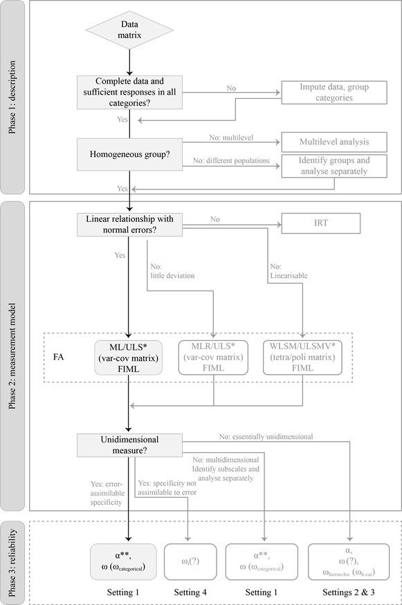
From what was elaborated up to this point it should have become clear that we discourage the analysis of the internal consistency reliability of a test by choosing the default instruction in the researcher's preferred software. On the contrary, we share with other works the idea that this analysis involves a complex but necessary process (Liddell & Kruschke, 2018; Savalei & Reise, 2019). We structure this process in three phases in which decisions are made successively: (1) the statistical description of the items; (2) the fit of the measurement model for the test and (3) the estimation of the internal consistency reliability of the test score(s). The focus of this paper is on the third phase, but, as we have seen, the reasoned choice of the reliability coefficient in this third phase depends on the decisions made in the first two phases. Therefore, some guidelines for addressing the first two phases are also given below. The three proposed phases are depicted in Figure 1. The vertical path highlighted and shaded in the left side of Figure 1 depicts the analysis that leads to the calculation of the coefficient α as recommended in the first line of Table 1, the most common scenario. The more complex alternatives discussed through this paper are depicted in lighter colour and without shading.
Phase 1: Statistical Description of the Items
The aim of this first phase is to gain knowledge about the distribution of item responses, to detect the possible presence of missing data, and to inspect the subgroups of persons and items for possible patterns that may illuminate the modelling to be carried out in the next phase.
Phase 1a: Data Completeness
The univariate description of the items provides information about the response distribution including possible missing values. If data are complete, it is possible continue with the analysis as planned. If some missing values are detected, it is recommended to use multiple imputation whether the data are analysed as quantitative (Ferrando et al., 2022) or as ordinal (Shi et al., 2020). Other possibilities are to use full information maximum likelihood estimation (FIML) during Phase 2 or to further refine the analysis according to specialised texts recommendations (e.g., Enders, 2010). All of these are better options than to eliminate cases with missing data from the analysis (listwise), or treat missing data based on bivariate information (pairwise) which is the default in some software. It is quite a different matter to observe categories with low endorsement or no endorsement at all. There is no way to infer this kind of non-observed responses and that may pose a problem for further analysis. To further analyse these data as categorical or ordinal the researcher may choose to collapse some nearby categories (e.g., Agresti, 1996; DiStefano et al., 2020). In previous phases of research, if the probability of endorsement of some response categories is very low in the population, you may consider gathering a very large sample of examinees or redesigning the response scale.
Phase 1b: Homogeneity of Persons and Items
Another task will be to assess whether the data come from a homogeneous population. If so, we can proceed with the analysis as planned. On the other hand, if the data collection design has been multilevel, it is advisable to deal with heterogeneity using multilevel analysis techniques (Cho et al., 2019; Hox et al., 2018). If the heterogeneity stems from data coming from different populations, one option is to continue the analysis for each group separately. If the underlying populations are not known, they can be identified by cluster analysis or even by latent class analysis as proposed by Raykov et al. (2019).
In addition, it is useful to inspect the homogeneity of the relationships between items. Heterogeneous relationships anticipate possible deviations from unidimensionality that will surface in the formal analysis in Phase 2. For quantitative data, the variance-covariance matrix (or Pearson correlation matrix) can be examined. For categorical or ordinal data, the tetrachoric (two response categories) or polychoric (more than two response categories) correlation matrix would be a better option. Visual inspection of these matrices may suffice if the number of items is moderate. More generally, the inspection can be conducted using multivariate statistical techniques such as exploratory factor analysis (EFA; e.g., Lloret-Segura et al., 2014), psychometric network analysis (e.g., Golino & Epskamp, 2017; see for practical application Pons et al., 2017), or multiple correspondence analysis (e.g., Greenacre, 2017).
The result of Phase 1 is a database for each population on which the test measurement model will be formally studied during Phase 2.
Phase 2: Analysis of the Measurement Model of the Test
The main objectives of this phase are to determine the dimensionality of the test as α and ω are only adequate for unidimensional measures, and to estimate the parameters involved in the calculation of ω.
Phase 2a: Specification of the Measurement Model
The first step is to specify a reasonable relationship between the items and the latent variables or factors. If the relationships are assumed to be linear and the residuals normally distributed, limited information estimation techniques can be used and the analysis in Phase 2b is simplified. On the other hand, if the relationships are specified as nonlinear, full information estimation techniques will be appropriate, the same techniques mentioned above for dealing with missing data.
If response categories are five or more it is reasonable to treat items as quantitative and linearly related to the latent variables as long as the responses to the items follow a normal distribution (Rhemtulla et al., 2012). In fact, they can be treated as normal if the absolute values of skewness and kurtosis are not greater than 1 (e.g., Ferrando et al., 2022; Lloret-Segura et al., 2014). When moderate deviations from normality are found, small corrections will suffice and will be discussed in Phase 2b. Otherwise, if extreme deviations are detected, such as those caused by floor or ceiling effects, a radical change of strategy should be considered. In this case, it will be advisable invoking other distributions of the residuals, such as the Poisson model (e.g., Foster, 2020; Muthén et al., 2016, cap. 7) or turn to non-linear models as described in the next paragraph.
In contrast, if items are answered in a response scale of four or less categories, a linear relationship with the latent variables is no longer reasonable and therefore it is preferable to treat the data as categorical or ordinal (Rhemtulla et al., 2012). The relationship can take several forms, but in the common case that researchers are interested in a two-parameter model (item difficulty and item discrimination), or the graded response model (difficulty of categories and item discrimination), then the relationships are linearizable by calculating polychoric or tetrachoric correlation coefficients. Otherwise, if researchers are interested in more complex models, for example, with more parameters, the alternative are the non-linear IRT models (Culpepper, 2013; Kim & Feldt, 2010).
A good practice is to specify all measurement models compatible with the theory underlying the construct, analyse them one after the other and choose the one that best fits the data and the purposes for which the test is to be used. When the test is intended to measure several constructs or factors, a typical sequence of nested models to check is (1) a flexible model allowing item cross-loadings between factors, and (2) a restricted model where factors are congeneric measures with no cross-loadings. If the test measures only one construct, the sequence is reduced to step (2) and perhaps to checking (3) the model of essentially tau-equivalent measures. On the other hand, if heterogeneity is suspected in the relationships between items of one construct, a reasonable sequence of models to check would be (1) a bi-factor model, (2) the congeneric measurement model and, perhaps, (3) the essentially tau-equivalent measurement model.
Phase 2b: Parameter Estimation and Model Fit
For parameter estimation, either item FA or non-linear IRT models can be used provided that data from large samples are available. Many cases can be solved through FA using either confirmatory (CFA) or exploratory (EFA) techniques (e.g., Bovaird & Koziol, 2012). In the simplest case, if the data are quantitative with item responses normally distributed, the use of the maximum likelihood (ML) estimator is recommended. As an alternative for slight deviations from normality, the use of the robust maximum likelihood estimator (MLR) is preferable. With ordinal data and a two-parameter model or a graded response model, the robust weighted least squares estimator with a χ2 statistic adjusted for mean and variance (WLSMV) is considered a suitable option. The general solution of estimating the parameters through full information maximum likelihood (FIML) can always be chosen at a higher computational cost.
If the sample size is small relative to the number of items, a preferable option for FA for quantitative data may be the unweighted least squares estimator (ULS; Ferrando et al., 2022) or for ordinal data the unweighted least squares with a χ2 statistic adjusted for mean and variance (ULSMV; Savalei & Rhemtulla, 2013). The number of cases that is considered a small sample size is a difficult topic but, as a guide, those analysed in the literature are in the order of 100 to 200 cases (e.g., Forero et al., 2009; Savalei & Rhemtulla, 2013).
The output of Phase 2 is the measurement model of the test that (1) is theoretically sound, (2) displays good fit to the data, and (3) displays better fit than alternative models compatible with theory. Typically, the output will be either a unidimensional model, an essentially undimensional model or a multidimensional model.
Phase 3: Estimation of the Internal Consistency Reliability of the Score(s)
As seen in the previous sections, the internal consistency reliability of the score of a test with unidimensional structure and specificity assimilable to measurement error can be obtained either using α or ω, that will provide close values. Researchers may also choose to report both types of coefficients. Conversely, if specificity is considered as true variance, the coefficient ωi will better reflect the reliability of the test score.
On the other hand, if the measurement model is multidimensional, α and/or ω can be calculated for each factor separately. When the model is essentially unidimensional our recommendation would be to clarify whether to consider the entire non common part as measurement error, which would be more consistent with reporting the coefficient ωhierarchical, or whether to consider minor factors as true variance which would be more consistent with reporting ω or even α. It may also be useful to report both types of coefficients (e.g., Green & Yang, 2015).
Finally, in all cases, it is good practice to report the confidence interval of the chosen internal consistency coefficient(s) or to report the Bayesian estimation of these coefficients (Pfadt et al., 2022). If the researcher chooses alternative coefficients that are beyond the objectives of this work, we recommend consulting specialized literature. This would happen, for example, with the coefficients derived from IRT or multilevel analysis, among other (Cho, 2022).
Computer Software for Internal Consistency Reliability Estimation
In this section, we present the current possibilities of widely used software to perform the three-stage analysis outlined above. In most cases, the analysis can be fully developed using one or, at most, two of them. We present open-source software R, Jamovi and JASP, and commercial software Mplus, SPSS and Stata. Jamovi, JASP, SPSS and Stata are menu-driven and can be complemented with syntax, while syntax is always required in R and Mplus. Our comments below refer to the analyses that can be managed through menus or syntax, explicitly ignoring the possibility of programming new functions. Figure 2 summarises this information.
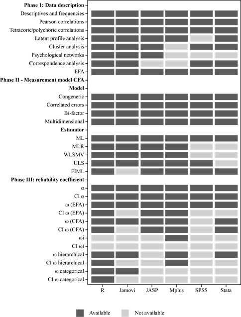
Note. EFA = Exploratory factor analysis; CFA = Confirmatory factor analysis; ML = Maximum likelihood estimator; MLR = Robust maximum likelihood estimator; WLSMV = Weighted least squares mean and variance corrected estimator; ULS = Unweigthed least squares estimator; FIML = Full information maximum likelihood estimator; tetra/pol = tetrachoric or polychoric correlations; α = Cronbach's alpha; ω = omega; ωi = specificity-corrected omega. CI = confidence interval.
Figure 2. Comparison of the Analytical Possibilities of Software to Complete the Three-stage Analysis for Reliability Estimation.
R (R Core Team, 2021). The data analyst can perform all the analyses we have suggested for each of the three phases (i.e., descriptive analysis of the items, fit of the measurement model of the test, and estimation of internal consistency reliability of test scores except coefficient ωi). The most convenient way to obtain results in R is to adapt a ready-made syntax. The work of Viladrich et al. (2017) presents a guide and the syntax necessary to carry out Phase 2 and Phase 3 for unidimensional tests. Point and interval estimate of the omega coefficient are derived from CFA. Syntax of point and interval estimates for alpha coefficient is also provided. Complementarily, Viladrich and Angulo-Brunet (2019) presents the syntax for Phase 2 and Phase 3 to obtain ωhierarchical based on a confirmatory bifactor model. In all these syntaxes the reliability function, which is deprecated, can be replaced by the updated compRelSEM function. As we have already said, if a multidimensional model is analysed, the reliability of each factor can be obtained separately and thus, the procedure proposed in Viladrich et al. (2017) for unidimensional tests can be applied to each factor. In addition to the confirmatory analyses, the package psych (Revelle, 2022; Revelle & Condon, 2019) allows to obtain α, ω and ωhierarchical based on the exploratory bifactor model, which by default assumes three minor factors. This exploratory option is not advisable (Savalei & Reise, 2019) due to the fact that it can lead to reliability overestimation based on non-plausible model results. To the best of our knowledge, no R syntax for ωi has been published so far.
Jamovi (The Jamovi Project, 2021). All the analyses proposed for Phase 1 can be carried out through menus. All the measurement models we have dealt with in Phase 2 can be analysed downloading the complementary module semlj (Gallucci & Jentschke, 2021) which installs the SEM menu. In Phase 3, with the SEM menu, you can get α, and the same ω options offered by the R package psych nowadays. Some particularities of this module are that it does not implement the FIML estimator and that with categorical data it calculates the ordinal version of α (Zumbo et al., 2007). We discourage the routine use of the pre-installed Factor menu. Although it offers CFA and EFA for quantitative data, and the reliability analysis option calculates the α and ω coefficients, it should be kept in mind that omega in the output is only correct for the congeneric unidimensional model, which is the default and cannot be assessed or modified by the user.
JASP (JASP Team, 2022). All statistical techniques mentioned in Phase 1 except correspondence analysis are available in JASP menus. In Phase 2, all measurement models can be tested with the Factor menu if an exploratory strategy is chosen or with the SEM menu if a confirmatory strategy is prefered. For Phase 3, the menu SEM provides point and interval estimation of α and ω. However, ω is only correct for the unidimensional model with maximum likelihood estimation which is the default and cannot be modified by the user.
Mplus (Muthén & Muthén, 2017). This commercial software offers the widest range of options for fitting the measurement model (Phase 2) and the first descriptive phase is also possible, except for multivariate techniques with no latent variables, such as cluster analysis, psychological network analysis and multiple correspondence analysis. Again, the most convenient option is to adapt ready-made syntaxes. Viladrich et al. (2019) provide a guide and the syntax for fitting the measurement model and estimating the reliability of unidimensional tests using CFA. For bifactor confirmatory models, see Viladrich and Angulo-Brunet (2019), for bifactor exploratory models see García-Garzón et al., 2020. For the computation of ωi see the syntax published by Sideridis et al. (2019). At the moment, we have not found published syntax to calculate directly ωcategorical in Mplus. Indirect options include copy-paste output values from Mplus to SAS (Yang & Xia, 2019) or export output from Mplus to R using the function mplus2lavaan from the package MplusAutomation (Hallquist et al., 2022; syntax available in Viladrich et al., 2019).
IBM SPSS (IBM Corp., 2021). All statistical techniques in Phase 1 are available through menus except for psychological networks and latent class analysis. The extended command SPSSINC_HETCOR downloadable from IBM developerWorks allows the calculus of tetrachoric and polychoric correlations using an R package. Other options include the syntax by Lorenzo-Seva and Ferrando (2012; 2015). Measurement models in Phase 2 can be fitted using IBM SPSS AMOS (Arbuckle, 2014), an additional software for structural equation modelling with a limited number of the estimation methods mentioned in Phase 2. For Phase 3, the command reliability of the core module provides the point estimation of α and, since version 27.0, also of ω for unidimensional models which is the default and cannot be modified by the user. As an option in the reliability command, point and interval estimation of α can be obtained as the intraclass correlation called consistency coefficient for average measures.
Stata (StataCorp, 2021). All statistical techniques in the descriptive phase are available except for psychological networks. The analysis of measurement models is generally performed with FIML estimation. In the third phase, Viladrich et al. (2019) provide syntax that facilitates the point and interval estimation of the coefficients α and ω for unidimensional models, whereas Viladrich and Angulo-Brunet (2019) provide syntax for bifactor models and ωhierarchical. To the best of our knowledge, the syntaxes for the calculation of the coefficients ωcategorical and ωi are not available at present.
Discussion
In this paper we have reviewed the current knowledge, practices and solutions concerning the estimation of the reliability of test scores based on an internal consistency design. The main results from our review are presented as a flow-chart aimed to help data analysts and paper reviewers. The flow-chart facilitates the reasoned choice of the reliability coefficient for scores obtained by sum or average of items with dichotomous or polytomous ordered category response scales.
Our first conclusion is that the classical α derived from the variance-covariance matrix between items performs well in most cases. We are more optimistic than Bentler (2021) when he concludes on the uses of α by a laconic "That's nice. But that's it. And it's not a lot" (p. 866). In our opinion it is quite a lot, at least by comparison with the uses of its best positioned competitor ω, although it is not enough because neither of the two coefficients provide a correct estimation of reliability in all cases. In fact, there is not a single coefficient that can do this job in all cases (Cho 2022; Xiao & Hau, 2022).
We consider it quite a lot due to compelling evidence in support of the close performance of α and ω when the data are approximately unidimensional the measures are congeneric with no extreme factor loadings and samples are large. Either coefficient would be correct in this scenario. And both would be incorrect for measurement models with correlated errors or items with a strong specific component.
Studies comparing α and ω under different conditions show that, in many cases, the difference between the two values is minimal. In our review we found that the conclusions in favour of ω in simulation studies are exaggerated as, under reasonable population reliabilities, the difference between the two coefficients reflects form the third decimal place onwards. This adds to the Savalei and Reise's (2019) conclusions that McNeish (2018) exaggerated the difference between the two coefficients and that the consequences of the divergence for practical purposes would be trivial.
In addition, using ω entails some dangers. The most serious stems from the subjective decisions involved when fitting the measurement model. Subjectivity can lead to much more inadequate results and make replication difficult (Davenport et al., 2016; Edwards et al., 2021; Foster, 2021), not to mention the bad practice of selecting an atheoretical but statistically fitting measurement model obtained from refinement based on the results. In our opinion, the best way to deal with this danger is to make all stages of the analysis transparent, including the availability of the database and the syntax used for the analysis.
Thus, in front of proposals that only advise the publication of some form of ω (e.g. Flora, 2020), we consider that α is appropriate in a wide variety of situations. We see coefficient α as simple to calculate, communicate and replicate, and differing from ω to the third decimal place in simulation studies, so with practical utility without a substantive loss in the rigour of reliability estimation. Let's wait and see if this conclusion is further supported by the replication of simulation studies in the future as proposed by Cho (2022).
For now, the most conservative position would be to report α and ω, as proposed by Revelle and Condon (2019). The publication of α will facilitate direct comparison with other studies (in fact, α is still the most reported reliability coefficient). Additionally, the publication of ω will provide an estimation based on the measurement model. If the difference between the coefficient α and ω was relevant, it would be worth discussing the reasons for this difference.
It should also be clearly stated that both coefficients share several limitations. To begin with, neither of them is useful for estimating the internal consistency reliability of scores derived from non-linear measurement models or with residual distributions largely departing from normality. For these cases, coefficients derived from linearised measurement models such as ωordinal (Zumbo et al., 2007) and ωcategorical (Green & Yang, 2009) have been dealt with in this text, but researchers should also consider coefficients derived from IRT models (Culpepper, 2013; Kim & Feldt, 2010) or Bayesian estimation applicable to a wide variety of exponential distributions (Foster, 2020, 2021) which have not been discussed in this text.
Furthermore, the use of α and ω is limited to the estimation of the reliability of scores obtained by item sum or average. The generalisation of these coefficients to estimate the reliability of factor scores can be seen in Rodriguez et al. (2016b) and in Ferrando and Lorenzo-Seva (2016, 2018). These papers address an even more important issue, namely the discussion of the psychometric usefulness of reliability coefficients compared to other indicators of the quality of factor scores such as factor determinacy and the common variance explained by the general factor. This is a very relevant practical issue because in popular analyses with structural equation models, the measure of latent constructs is not obtained by item sum or average, but by factorial combination of item responses. In short, although the extreme positions of the letters α and ω in the Greek alphabet suggest that they are coefficients located at antipodes, evidence show that they solve quite the same psychometric issues.
Another important point for practical purposes is that there are no shortcuts to calculate α and ω. Indeed, one idea that has survived the discussion of coefficients over the last few decades is that whatever coefficient is used, the estimation of the internal consistency reliability comes after testing the measurement model. This idea is now well-established and included in normative texts such as the publication manual the American Psychological Association (2020) or the methodological quality guidelines for meta-analysis (Prinsen et al., 2018; Sánchez-Meca et al., 2021). In other words, before calculating the internal consistency reliability with α or ω, it must be checked that a FA of the items show results compatible with the CTT. And we add that the right type of FA should be determined through the previous exploration of the data. Our view of the analysis as a three-stage journey is aligned with scholars that affirm that there are no quick ways to calculate internal consistency reliability (e.g., Liddell & Kruschke, 2018; Savalei & Reise, 2019) and far from the point of view of other scholars who advocate for the dissemination of specific software that produces a proxi for ω in a few steps avoiding the assessment of the measurement model, as for example can be done the macro by Hayes and Coutts (2020) for SPSS. As simulation studies have shown, in most cases, a good proxy for ω is simply α.
In this area, our specific contribution consists of pointing out that not only the road is long but, in their curves, researchers will find unexpected species in point-and-click-psychometrics such as cluster analysis, making decisions about the expected relationship between items and factors, about what parts of the variability of the responses are going to consider true or error variance, or what is a reasonable form for the distribution of the residual variance. The reward will be a deep knowledge of their data, the human group who participated and the theory underlying their test.
Another risk is to think that the empirical demonstrations on the utility and efficiency of ω for unidimensional quantitative data are generalisable to any other version of the coefficient ω, as for example, is implicit in the work by Flora (2020), in Lai (2021) or in Bentler (2017). These papers introduce new coefficients based on ω and usually provide a computer solution to calculate them. On the one hand, the warning by Revelle and Condon (2019) against the temptation to apply reliability formulas to tetrachoric or polychoric correlation matrices and, for the other thing, the debate about coefficient ωordinal (Chalmers, 2018; Yang & Green, 2015; Zumbo & Kroc, 2019), has made us more cautious about jumping to conclusions relative to new coefficients. That is why we have changed our mind with respect to our previous work (Viladrich et al., 2017). We now believe that mathematical generalizations of ω to new analytical conditions should be accompanied by comparative empirical investigations, such as that by Yang and Green (2015) or the more recent by Béland and Falk (2022) showing their advantages.
As far as the software is concerned, the implementation of the coefficient ω is widespread while that of the coefficient ω is more restricted. If the data and model characteristics are aligned with the shaded path in Figure 1, the choice of software will not be a major problem for ω and even less so for α, since both coefficients are generally available. As the characteristics of the data or model move away from the ideal shaded in Figure 1 (e.g, the relationships are non-linear, there are some correlated errors, data are ordinal) the need to calculate a particular type of ω will also require access to and knowledge of specialised software packages. We want to warn against the unthinking use of software under the heading reliability or similar. Some of these, such as the Factor reliability menu of Jamovi, the reliability menu of JASP or the omega function of the psych package in R, provide reliability results without the user having control over the measurement model, whereas the measurement model is of utmost importance as the numerator of ω is based on factor loadings. It should be noted that, for the time being, these solutions are based on unidimensional EFA and would only be appropriate when the data display the conditions shaded in the left of Figure 1. Additionally, documentation regarding methods underlying an option in the menu is generally difficult to follow, the exception being the well documented psych package (Revelle & Condon, 2019). Instead, we favour the use of functions such as compRelSEM from the semTools package in R that derive the calculation of reliability coefficients from the parameters estimated when fitting the measurement model. In other words, when data departs from the shaded path in Figure 1, researchers and reviewers should only trust functions where ω is a subproduct of a factor analysis defined by the data analyst and not obtained as a default in a statistical software.
Consistent with this, some comments on methods for reliability generalisation meta-analysis are in order. As we have said, we share the indication that the measurement model should be taken into account. However, once the unidimensional model has been fitted, the aggregation of reliability results is done without distinguishing between its estimators whether they are α or ω (Julio Sánchez-Meca et al., 2021) or only α (Prinsen et al., 2018). Perhaps not distinguishing between α and ωtotal might be a good idea since both coefficients share the definition of true variance and thus, aim to estimate the same population parameter. On the other hand, we consider results obtained with ω hierarchical or with ωi as not aggregable either with each other or with α and ωtotal, since the true variance is defined in a non-comparable way. Therefore, they should be treated separately, as it is common practice with other coefficients that not share with α the definition of true variance such as the intraclass correlation coefficient of absolute agreement (Prinsen et al., 2018). We think that in all studies should be explicitly reported which part of the variance of the responses has been considered as true variance. In this vein, Cho (2022), reaches a similar conclusion, and Scherer and Teo (2020) propose the more drastic solution of performing reliability generalisation meta-analyses on the basis of the variance-covariance matrices and not on the basis of the coefficients reported in the primary studies. This type of analysis, named meta-analytic structural equation modelling or MASEM, is developing very fast for the study of reliability generalization (Sánchez-Meca, 2022).
Turning to the study design and data analysis, researchers must go beyond the mental framework of obtaining data with a single administration and consider a posteriori which is the best formula for estimating internal consistency reliability. In fact, it is necessary to be clear from the outset about all sources of variation to include them in the data collection design. For example, if the researcher wants to measure a conceptually broad construct with few items, those items will have sizeable specificity. This knowledge will allow them to design the data collection in such a way that it is possible to estimate it and include it as true variance (Bentler, 2017; Raykov, 2007). Or perhaps a researcher may choose to include some sources of error in the analysis of the measurement model as is done for example in the work of Ferrando and Navarro-González (2021) who, using a cross-sectional design, propose a data analysis model in which the error attributable to each person is estimated in order to quantify the role it plays in the reliability of a test.
As novel as these proposals may seem, in our view, they add to what was and continues to be the objective of GT since the fifties of the last century. As we have said, from this theory, the study of reliability is conceived as the identification and control of possible sources of error in test scores. The designs and analyses proposed by Bentler (2017), Ferrando and Navarro-González (2021) Green and Hershberger (2000) or Raykov (2007) simply promote the statistical control of the sources of error in front of the experimental control initially adopted in GT.
We think that addressing the question of how to control or at least predict possible sources of error helps to address a well-known handicap of all reliability coefficients. These coefficients depend not only on the test but also on the group of people to whom it is applied and on the test correction procedure. According to Ellis (2021) one way to deal with this situation is to explicitly recognise that the same test can have multiple reliabilities. That is, now that we have accepted that there is no single formula for estimating reliability, and that the best formula will depend on what is considered error for each intended use of a test, we have taken the first step in admitting that there is also no fixed number of designs to cover this purpose. For each proposed use of a test it will be necessary to justify what evidence of reliability would be compelling as recommended by Muñiz and Fonseca-Pedrero (2019), Ziegler (2020) and, reflected in the different groups of reliability evidence collected in the Standards for Educational and Psychological Testing (AERA et al., 2014). This point of view entails a clear extension of the three classic designs of internal consistency, test-retest reliability and parallel measures, and consequently also of the interpretation of the resulting coefficients.
A final recommendation for editors and reviewers would be that in addition to assessing the choice of coefficient, importance should be given to the acceptable cut-off points and the report of confidence intervals. This message is not new, but we repeat it because it seems to be difficult to apply. Although many authors have provided cut-off points for reliability coefficients (see, for example, (DeVellis, 2003; Nunnally & Bernstein, 1994; or more recently Kalkbrenner, 2021; Taber, 2018), mainly based on personal opinions (Streiner, 2003), the proposal of Nunnally and Bernstein (1994) is the most recognised. For example, the recommendations of the COTAN model are explicitly based on it COTAN (Evers et al., 2013). Nunnally and Bernstein (1994) based their proposal on the use of test scores and established two uses: using the scores to obtain correlations with other variables or using them to make assessments of individuals. In the first case they set a reliability cut-off point at .80 to ensure that loss of reliability in the measures did not lead to a large attenuation in the correlations. In order to obtain highly accurate measures for the second use they raised the minimum reliability value to .90. However, these authors are often cited to justify reliability values of .70, when they restrict this value to "early stages of predictive or construct validation research" (p. 264). Although it does not follow from their recommendations that any of these values should be taken as absolute benchmark, nor are these recommendations supported by empirical studies, many researchers, reviewers and editors resort to them, especially the lower criterion of .70, as absolute cut-off points (Cortina et al., 2020; see also Lance et al., 2006). It is also striking that it is common to provide point estimates of the coefficients, either α or ω, without the confidence interval of the coefficient as an indicator of the level of precision of the estimate, which should be standard practice for sample estimates as claimed in normative texts (Evers et al., 2015; Prinsen et al., 2018; Sánchez-Meca et al., 2021). It must be acknowledged that the value that should exceed the cut-off point is the lower limit of the confidence interval. An alternative treatment of uncertainty is that proposed in Pfadt et al. (2022) based on Bayesian estimation of these coefficients.
In a nutshell, if you plan to study the internal consistency reliability of a test score, it would be advisable to (a) organize the data gathering to include variables to account for all known sources of error; (b) analyse data exploring their completeness, shape, and relationships and test the measurement model fit; (c) report the interval estimation of the reliability, using α or other coefficients; and (d) gauge its value depending on the intended test use.
This paper does not intend to close the debate on the use of internal consistency coefficients, much less on the estimation of reliability. At present, the debate is so rich and wide-ranging that addressing all its extremes would require much more space than is available in this paper. Moreover, as can be seen from the references, this is a field in continuous development to which much attention will have to be paid in the future.

