INTRODUCTION

Overweight and obesity (OW + Ob) have become critical issues in the recent decades. Between 1990 and 2022, obesity prevalence among adults has increased by over 20 % in 45 countries, based on age-standardized data from recent studies. This issue extends beyond adults and significantly affects school-age children and adolescents (5-19 years). For girls, 186 countries (93 %) reported an increase in obesity, whereas for boys, this increase was observed in 195 countries (98 %). Many countries registered a twofold increase, with notable increases in Polynesia, the Caribbean Islands, Brunei, and Chile (¹). Epidemiological changes associated with nutritional transition have been studied for decades. Since 1993, Dr. Popkin (²) and current studies conducted in 2019 (³) and 2024 (¹) have documented trends and proposed behavioral patterns that provide a complete overview of the slow and rapid increases in OW + Ob prevalence worldwide. While most regions show a steady rise, some areas with a high prevalence have stabilized. In Mexico, the rising prevalence of OW + Ob among children has serious consequences. Immediate health implications include a higher risk of chronic conditions such as type 2 diabetes, cardiovascular disease, and hypertension, which were previously seen mainly in adults but are now common in younger populations (⁴). Obesity also affects physical parameters such as motor performance and coordination, which are linked to regular physical activity and body composition in children and adolescents (⁵). Moreover, overweight and obese children often face social and psychological challenges, including stigmatization, bullying, and low self-esteem, which can have lasting effects on their mental health and wellbeing (⁶,⁷). The economic burden of obesity-related healthcare costs is substantial, placing strain on healthcare systems and contributing to socioeconomic disparities (⁸). Furthermore, obese children are more likely to remain obese during adolescence and adulthood, thereby perpetuating the cycle of obesity and its associated health risks.

Between 2015 and 2018, Mexico conducted the National Registry of Weight and Height (RNPT) to collect anthropometric data from approximately 15 million school-aged children nationwide. In its first round (2015), with approximately 10 million anthropometries, the RNPT found a 34.5 % prevalence of OW + Ob (⁹). Further details on RNPT characteristics, coverage, and results are available in literature (¹⁰). In Mexico, the prevalence of OW + Ob among school-age children (5-11 years) has increased from 25.5 % in 1999 to 35.7 % in 2020, reflecting a 40 % increase over two decades (¹¹,¹²), and the most recent data from the National Health and Nutrition Survey (ENSANUT 2022) reported an OW + Ob prevalence of 37.3 %, indicating the trend continues. Anthropometry is indispensable for monitoring the nutritional well-being of children in developing populations (¹³), and the central role of nutritional status is critical for children’s overall health and well-being worldwide (¹⁴). Analyzing the OW + Ob trends during the school-age period is essential for understanding the patterns that lead to a high prevalence of 41.2 % in adolescents (12-19 years) and 75.2 % in adults in Mexico (¹⁵). The prevalence among preschool-age children (0-4 years) is 7.7 % (¹⁶), with a cut-off for OW + Ob at ≥ 2 Z (¹⁷); however, when using the cut-off for ages 5-11 years at ≥ 1 Z, the 2022 prevalence of pre-school children was 26.1 % (¹⁸). When analyzing the prevalence of OW + Ob among populations, we sought to understand some of the differences present in specific population subgroups and geographic, cultural, and social characteristics. These elements are important guides for future research, particularly to improve the prediction of future trends. These changes over time stress the importance of analyzing the behavior of the data to compare the magnitude of this phenomenon among populations and over time.

Our working group developed a polynomial model to analyse pairs of data on age in months and BMI Z in the period 60-144 months, using the polynomial index of overweight and obesity (IPSO). This index, similar to the one previously developed to assess malnutrition in children aged 0-4 years (¹⁹), will facilitate comparisons of OW + Ob in different populations and time periods. Examples of other public health indices that use anthropometric data include the Global Hunger Index (https://www.globalhungerindex.org) and Global Obesity Observatory (https://data.worldobesity.org/).

The main objective of the present work is to test the developed model for three different scenarios: first, as an easy method to compare and diagnose the OW + Ob magnitude among populations; second, as a comprehensive and visually clear tool to characterize the evolution of OW + Ob development during the school-age time lapse; and third, as a reliable tool to rapidly compute indexes, inspect, analyze, and compare the OW + Ob behavior of different subpopulations in response to variables of interest.

MATERIAL AND METHODS

Input data and polynomial function calculations

To model the behavior of OW + Ob in a population during the 5 to < 12 years old time lapse, we proposed using data pairs consisting of the population’s means of age and the z-score of BMI/age defined by the WHO (²⁰) for each of the 7 year intervals in months: [60, 72], [72, 74) up to [132, 144] using the ages in the X axis and the z-score in the Y (Table IA).

Table I Data for polynomial algorithm 

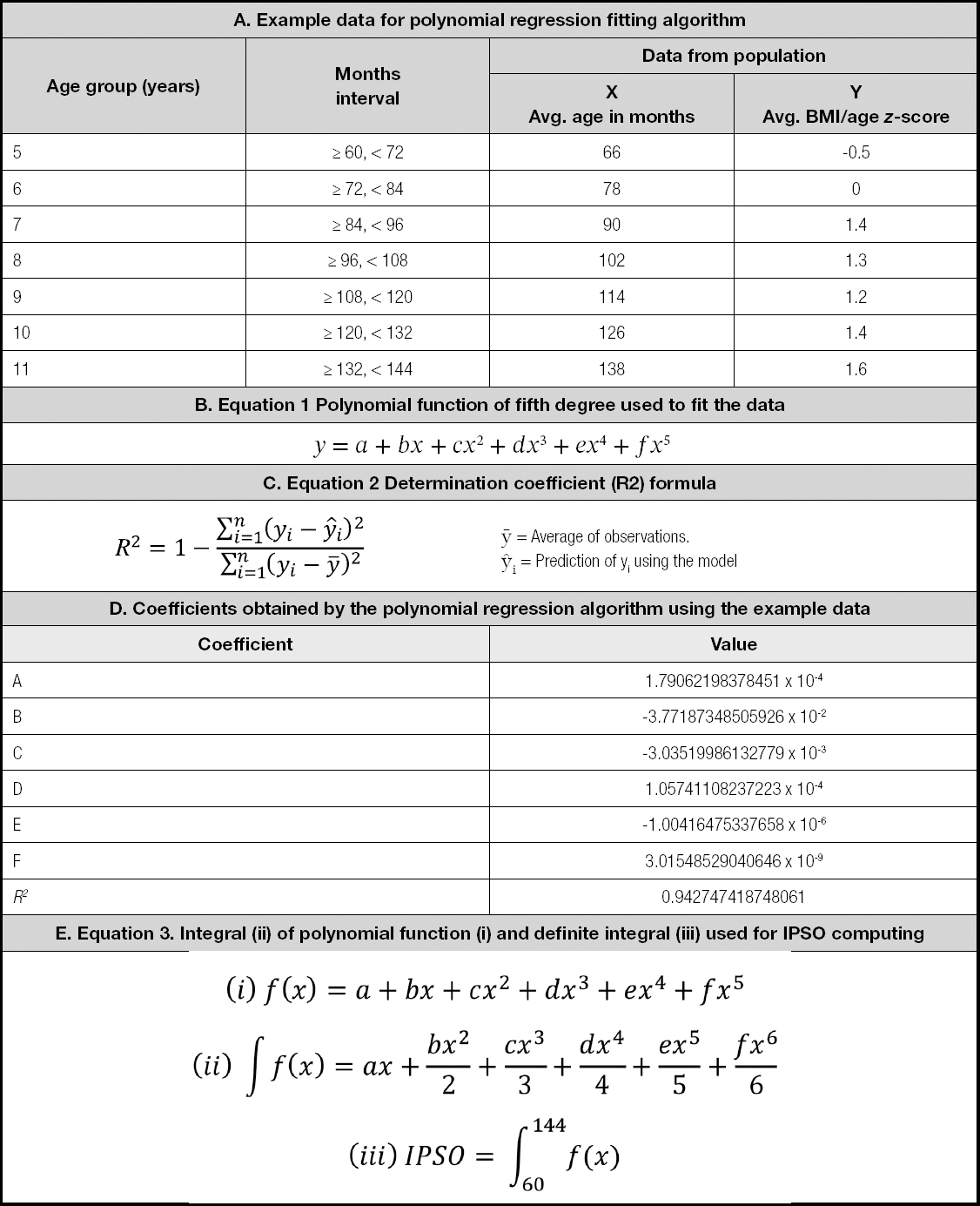
The model justification lies in the fact that this polynomial model represents a curve that describes how the variable of interest (z-score average) that represents the BMI/age status of the population behaves through the 5-11 years old time lapse. In other words, the area under this curve could be interpreted as the OW + Ob magnitude of the population over time.

To model this data, we developed a polynomial regression algorithm in the Transact-SQL language for implementation on a Microsoft SQL Server database. This algorithm was designed to obtain n + 1 coefficients of an n-order polynomial function when n + 1 (x,y) data pairs are provided (²¹). In the present work, a fifth-degree polynomial function (Table IA) was chosen because of its precision in modelling up to five inflection points using six coefficients (A to F).

In order to validate how accurate was the fitting process, along with the calculation of the coefficients, an additional function was written to obtain the “determination coefficient” also known as R2 (Table IC), which expresses the goodness of fit of the model. This value ranges from zero to one. When these values are closer to one the model fits the data better. Additionally, because the intended use of the model is based on data from populations, one may expect to have sufficient observations in each group, thereby avoiding large fluctuations in the Z-averages due to a small n effect, leading to smoother and better-fitted polynomial models. Considering these two conditions, we expected that the IPSO would perform well when estimating the OW + Ob magnitude.

For the data in table IA, the coefficients and R² values were obtained when the polynomial regression algorithm was applied. The coefficients and R² values were obtained for the data in table ID, when the polynomial regression algorithm was applied.

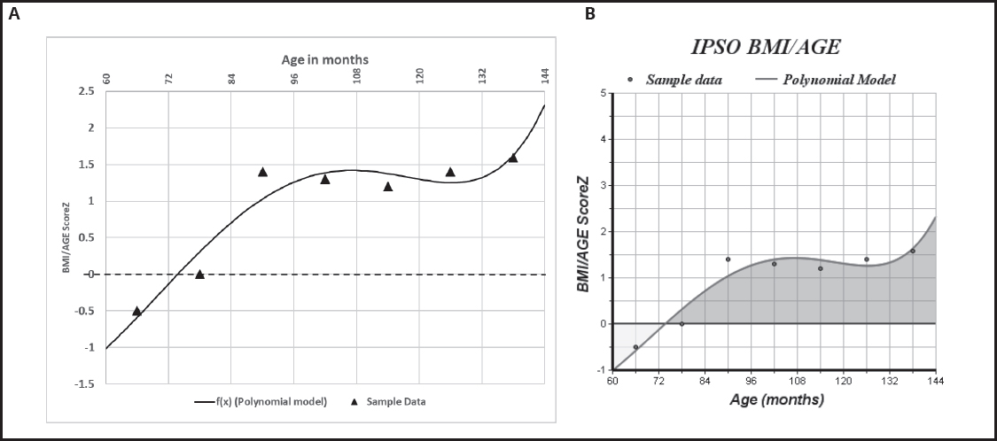
Replacing coefficients in Equation 1 and evaluating the function in the 60-144 months interval allowed us to plot the model vs. actual sample data to evaluate the behavior of the modelling process (Fig. 1A).

Figure 1 Examples to visualize IPSO algorithm. A. Actual sample data (black triangles) vs polynomial model (black line) obtained by the polynomial regression algorithm. B. IPSO plot generated by the calculation website. 

IPSO USAGE AND TESTING WITH ANTHROPOMETRIC DATA FROM NATIONAL SOURCES

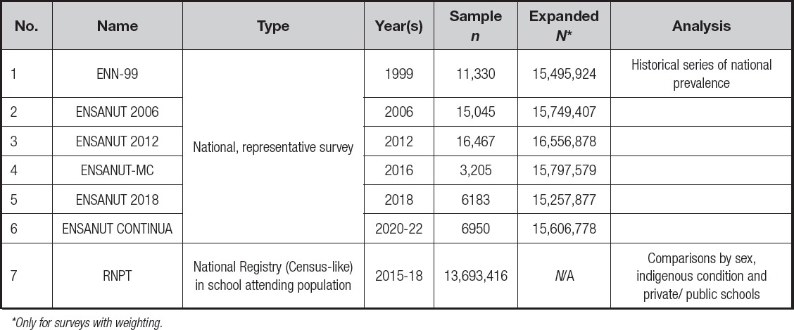
We evaluated anthropometric school-age children´s data from the 1999 National Nutrition Survey (ENN) (²²), National Health and Nutrition Surveys (ENSANUT) from 2006 to 2022 (¹⁸), and National Weight and Height Registry (RNPT) from 2015 to 2018 (²³). Table II presents the main characteristics of the datasets used in this study. In all surveys, a clustered and stratified sampling design was used to calculate the age and score-z means. All data were included in the RNPT case. All analyses were conducted using SPSS version 27.0, and the resulting means were used in polynomial regression and definite integral tSQL scripts to obtain the models and indexes, respectively.

Table II Datasets used for IPSO testing and its main characteristics 

*Only for surveys with weighting.

WEBSITE INTERFACE AND PLOTTING DEVELOPMENT

A website was developed to provide an open-access online tool to anyone who wants to analyze their own data by implementing the algorithms. To host the site, Windows Server 2012/IIS 8.0 and Active Server Pages (ASP Classic) language were used along with the SQL Server database. To provide visual support to the IPSO calculation, the Chart Director plotting library (²⁴) was implemented to display the sample data, model, and area under the curve that represents the IPSO (Fig. 1B).

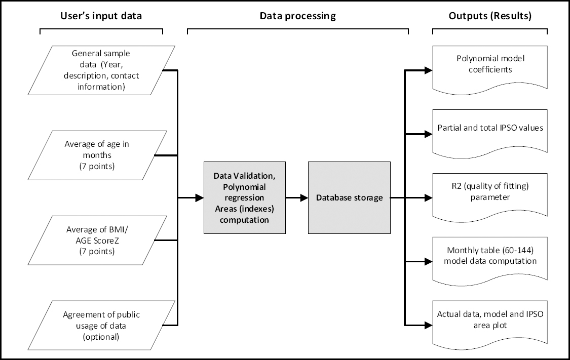
This site can be accessed at https://ipso.slan.org.mx, on it user is requested to input the 7 data pairs as well as general information regarding its data. When a user submits their data, the IPSO index, polynomial function coefficients, model data, R², and plot are obtained. When entering data, the user can choose to make it public or keep it confidential; thus, the IPSO website also serves as a data collection repository for OW + Ob prevalence from many sources and users. A diagram summarizing the operation of the IPSO website is shown in figure 2.

Figure 2 User inputs, processes and outputs of IPSO website. 

RESULTS

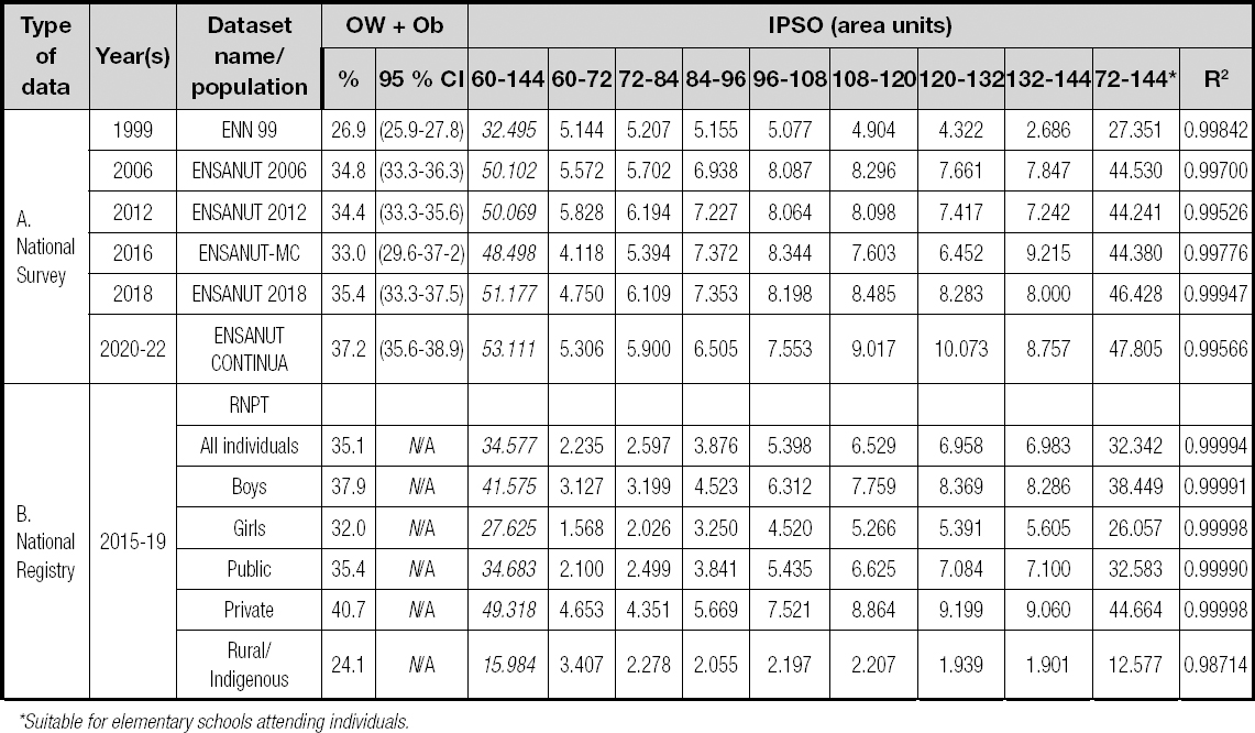
Table III presents the prevalences of OW + Ob, the global and partial IPSO values and R² values for the present study datasets, i.e., the coefficients of fetermination (R²) for the models. The table shows a comparison and magnitude between the OW + Ob prevalence and global IPSO values. Our results cover our first scenario as a simple method to compare and diagnose the magnitude of OW + Ob between populations. In a normally distributed population, approximately 16 % of the individuals are expected to be above one standard deviation (classified as OW + Ob), which is important for making comparisons and decisions. IPSO values near zero are typical for normal populations, so any positive IPSO value indicates an OW + Ob magnitude, facilitating comparisons between different groups.

Table III Prevalences of OW + Ob, global and partial IPSO values and R² values for the present study datasets 

*Suitable for elementary schools attending individuals.

The OW + Ob magnitude obtained through IPSO_60-144 was 32.5 % for the initial survey (1999), after which an important increase led to 50.1 % in 2006. From this point, a constant increase continued until it reached a peak of 53.1 in 2022 (Table IIIA).

As explained previously, the second scenario was to verify whether the IPSO was capable of evaluating the OW + Ob behavior in different age groups, thus allowing the identification of the magnitude behavior inside and between every year of the school-age period. Regarding this, one can see that between 1999 and 2012 all partial IPSO’s increase, in the 60-72 months group the shift is from 5.14 to 5.82 area units (+13.2 % relative increase), this contrast remarkably with the 132-144 group age, that passes from 2.68 to 7.24 area units (+170.1 % relative increase)! (Table IIIA).

The RNPT transversal data (Table IIIB) demonstrate that IPSO can detect differences in OW + Ob magnitude related to population characteristics such as sex and socioeconomic status. For instance, girls had an IPSO of 27.62 area units, while boys had 41.57 for a general (IPSO_60-144) index value (Table III). The notorious differences in IPSO values by the variable of interest (sex in this case) were precisely the third scenario of the main objective of present study. The period between 84-96 months (7-8 years) showed a significant rise in OW + Ob for both sexes, with 96-108 months period (8-9 years) also marking critical increases (Fig. 3C).

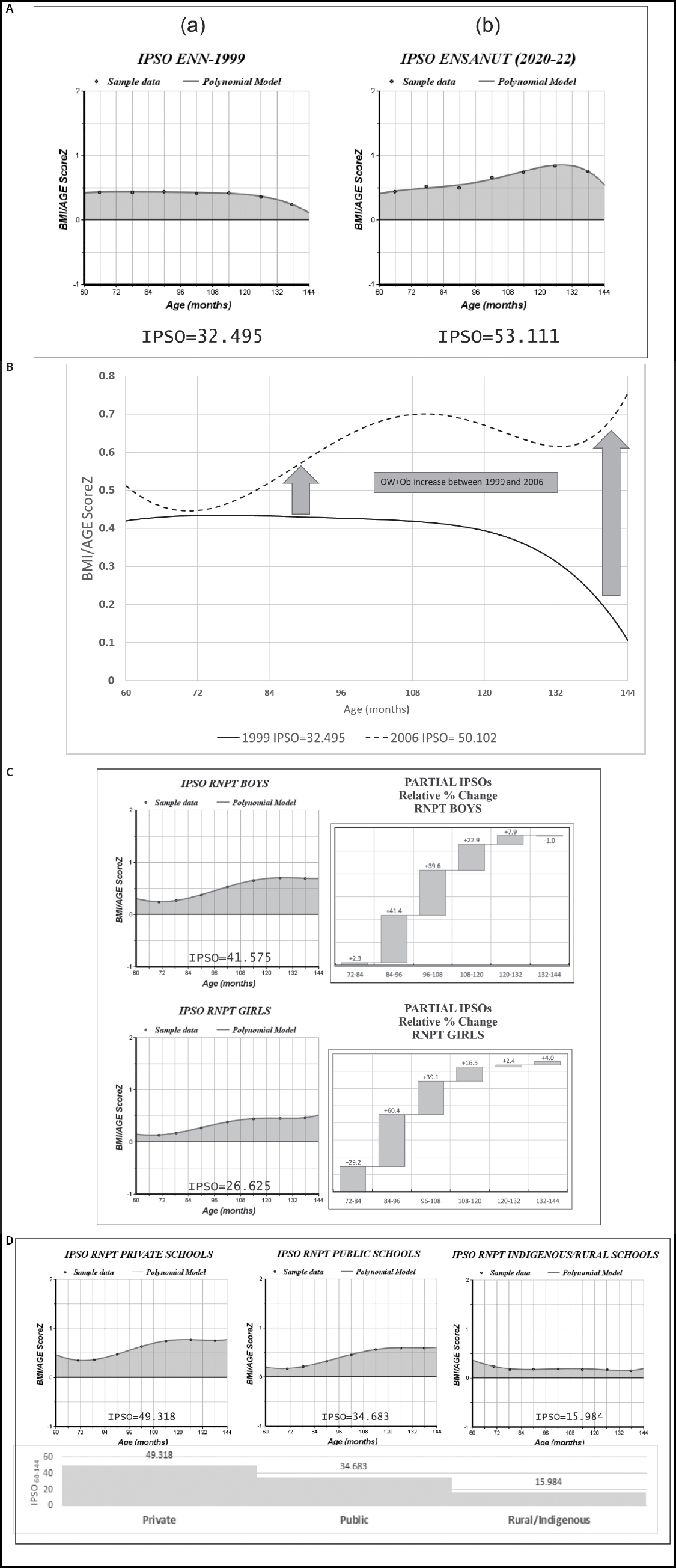
Figure 3 Comparison of IPSO results. A. Comparison of IPSO plosts for ENN 1999 vs ENSANUT CONTINUA 2020-2022 (continues on next page). Comparison of IPSO results. B. Polynomial models data comparison between 1999 and 2006 surveys. C. IPSO plots and cascade charts representing the partial IPSO relative percentual change in boys and girl’s populations from RNPT (continues on next page). Comparison of IPSO results. D. IPSO plots and values of RNPT private, public and rural/indigenous schools and bar chart of IPSO values corresponding to each population. 

Changes over time can also be visualized through IPSO, an example of which is the comparison of the National 1999 and 2022 surveys (Table IIIA), which passed from 32.495 to 53.111 area units in such a time lapse, representing a relative increase of 63.4 % in the OW + Ob magnitude, which cannot be detected using the raw prevalence comparison. The shift from 26.9 % to 37.2 % corresponds to a 38.8 % relative increase, thereby underestimating the changes.

This relative OW + Ob increase of 63.4 % between the 1999 and 2022 surveys can also be easily observed in the graphs produced by the IPSO website; in figure 3A, the graphics show the actual data pairs (points), the polynomial model as a line, and the area under the curve (orange shaded area) representing the IPSO_60-144 model.

A two-sample Mendelian randomization analysis discerns food intake causally linked to CVDs: heart failure (HF), atrial fibrillation (AF), dilated cardiomyopathy (DCM), and coronary artery disease (CAD) (Aao: ascending aorta; Ao: aorta; Dao: descending aorta; DBP: diastolic blood pressure; Ecc AHA: peak circumferential strain according to the American Heart Association; Ell: longitudinal strain; Err AHA: radial strain according to the American Heart Association; LAEF: left atrium ejection fraction; LASV: left atrium stroke volume; LAV: left atrium volume; LVCO: left ventricular cardiac output; LVEDV: left ventricular end-diastolic volume; LVEF: left ventricular ejection fraction; LVESV: left ventricular end-systolic volume; LVM: left ventricular mass; LVSV: left ventricular stroke volume; max: maximum; min: minimum; PP: pulse pressure; RAEF: right atrium ejection fraction; RASV: right atrium stroke volume; RAV: right atrium volume; RVEF: right ventricular ejection fraction; RVEDV: right ventricular end-diastolic volume; RVESV: right ventricular end-systolic volume; RVSV: right ventricular stroke volume; SBP: systolic blood pressure; and WT AHA: myocardial wall thickness at end diastole according to the American Heart Association).

Since one of the IPSO’s website results consists in a monthly (x, y) data matrix, the data pairs of 60 to 144 ”x” values and the “y” predicted by the polynomial model can be used to plot several population models in a single chart. An example of this can be seen in figure 3B, in which the OW + Ob magnitude increase over seven years is clearly represented as the area between the solid (1999) and dotted lines (2026).

The prevalence of OW + Ob has increased in recent decades, particularly in developed countries (²⁵). These tools could help to document and measure childhood obesity as a major public health concern. In this sense, the proposed IPSO models performed robustly when comparing the OW + Ob magnitude between populations at the global level, and the partial indices and plots allowed us to describe and visualize the behavior of the OW + Ob phenomenon through school-age time lapse. In figure 3C, IPSO plots for boys and girls from RNPT are show side by side against the relative percentual change (RPC) of partial IPSO values for each population (Table III, columns 60-72 to 132-144) this RPC was defined as the “n” interval IPSO minus the “n-1” IPSO interval divided by the “n-1” IPSO. This relative change expresses how much the area has changed from one age group to the next as a percentage fraction of its initial state.

Figure 3D shows RNPT plots and data from three RNPT subpopulations: children from private, public, and indigenous/rural schools. This allows for a quick comparison between the different groups, which behaves as expected, with the children from private schools showing a greater IPSO value, whereas indigenous/rural ones (from the poorest communities) presented smaller IPSO values.

DISCUSSION

Through the development of a polytomous model, this research corroborated its estimation, application and use across different data sources to assess the relationship between age in months and body mass index (BMI) z-score for age in children aged 60-144 months. The results demonstrated the usefulness of the model for comparing the magnitude of overweight and obesity among different populations, constituting a visually clear and reliable tool for the analysis of indices in various subpopulations.

Although BMI does not directly express adiposity distribution, it is still used as one of the most important health parameters to evaluate OW + Ob. These conditions are recognized as serious threats to public health and are associated with chronic diseases and risk factors in terms of attribu table deaths and disability-adjusted life-years in the adult population (²⁶). For school-aged individuals, BMI is useful for assessing nutritional status during the growth period (²⁷), and the magnitude of changes in prevalence during this period is key to describing this phenomenon among populations over time (²⁸).

With the present work data we were able to identify using the IPSO an accelerated increase in OW + Ob magnitude around the age of 8 years, which led us to propose that this early age could be the best time for interventions aimed at addressing this problem in the population.

The results from the 1999 nutrition survey show a flattening and even a slight reduction in OW + Ob magnitude between 9 and 11 years of age; this behavior is also noticed in the upcoming surveys. Further research is needed on this behavior, such as the presence of early puberty, and its relationship with adiposity increases and growth rate decreases (²⁹).

Similar to our findings, which identified sex-typical behaviors and early onset of overweight and obesity, these findings have been documented by other authors. For example, a secondary data analysis was conducted in El Salvador in children aged 6 to 9 years, in which the authors reported a greater OW + Ob prevalence in 6 years old children (girls = 31.5 %, boys = 35.5 %) than in the 9 years old group (girls = 18.7 %, boys = 24.5 %) (³⁰). In China, a population analysis in children aged 6 to 11 years found an alarming increase in OW + Ob prevalence in the 1991-2011 period passing from 7.9 to 20.5 %; in this study, as in ours, boys had a higher prevalence of OW + Ob than girls (³¹).

For the analysis of behavior among other socioeconomic and sociodemographic variables such as rurality, characteristics and school environment, we identified that similarly, a study conducted in El Salvador, the authors detected a greater prevalence of OW + Ob in urban schools (girls = 35.1 %, boys = 38.9 %) and private schools (girls = 42.2 %, boys = 46.6 %) than in rural (girls = 23.6 %, boys = 26.6 %) and public schools (girls = 26.8 %, boys = 29.9 %) (³⁰). This behavior of a greater magnitude in OW + OB in schools from wealthier and more urbanized areas is consistent with the results obtained using our IPSO testing data and is usually related to a greater intake of high energy density products derived from non-healthy feeding patterns (³³) and a greater exposure to obesogenic environments (³⁴). Finally, a study conducted in England examined the relationships between socioeconomic variables, such as distance to supermarkets, income, population density, dwelling, employment, and education, with OW + Ob prevalence in the school-age population. The results showed that regardless of dwelling, a positive relationship was found between distance to supermarkets and obesity, as children from urban areas were slightly more obese than those from rural areas, with the exception of children from families with higher incomes in urban areas (³²).

The previous analyses and results obtained from several data sources allow us to propose IPSO as a novel tool for the epidemiological assessment of OW + Ob in school-age children, mainly because it proved to be effective when comparing populations, contrasting subpopulations based on variables, and describing OW + Ob behavior through the 5-11 years old timelapse. Among its strengths compared to other model types, the present study data showed that the prevalence of OW + Ob does not necessarily operate in a linear or exponential manner; in fact, such data tend to fluctuate between the age groups, and this is the scenario in which a 5th degree polynomial function performs better by modelling the inflection points in the data. However, the most important weakness is that a considerable number of observations are needed for each of the seven age groups to account for plausible prevalence values to compute the model. Another weakness is that, to date there is no extensive repository of IPSO values to compare the obtained results; however, this issue could be addressed gradually by spreading this index usage.

The use of standardized indices to evaluate populations provides results fundamental to public policy design and effect measurement. Furthermore, these results are essential for planning and focusing on actions to support highly exposed individuals.

CONCLUSION

The IPSO usage proposal as a standard to evaluate the OW + Ob magnitude in school-age populations proved to be useful when comparing them, as well as when inspecting the behavior of such magnitude over the age groups. The index also performed well when comparing multiple populations from several sources and was able to contrast them in a direct and visually simple way to diagnose many populations and evaluate the dimensions of the OW + Ob problem among them. The IPSO is a novel proposal that intends to contribute to existing OW + Ob surveillance and monitoring tools, such as the NCD Risk Factor Collaboration (³⁵,³⁶), WHO Global Health Observatory (³⁷), Global Burden of Disease Study (³⁸,³⁹), and Global Nutrition Report (⁴⁰). The IPSO is a tool that can be used in further research on OW + Ob magnitude in school-age populations and, in this way, contributes to direct or changing the recommendations about local interventions and public policies.