


 Servicios personalizados
 Inglés (pdf)
 Articulo en XML
 Referencias del artículo
 Enviar articulo por email
 Citado por SciELO
  Citado por Google
  Similares en
SciELO
Similares en
SciELO  Similares en Google
 Permalink
Observational methodology allows the spontaneous behaviors of participants in natural situations to be recorded and then quantified (Anguera et al., 2020). This methodology involves an initial phase based on naturalistic observation and a second phase involving a quantitative analysis of participant data. The final stage of observational methodology includes qualitative conclusions based on the first two phases. This type of methodology is used not only in psychology, but also in social research, education, sports, and health. Its multiple advantages include a low intervention level, independence from standardized measurement tools, and its applicability in atypical intervention contexts (Anguera et al., 2018; Chacón-Moscoso et al., 2014, 2018, 2021).
The term observational methodology is used in this paper to differentiate this methodology from observational studies in health. In that type of quantitative study, which can be cohort, case-control, or cross sectional (Cochran & Chambers, 1965), researchers track participants to identify cause-effect relationships when randomization and experimental control cannot be applied. Though the publication of tools like the Strengthening the Reporting of Observational Studies in Epidemiology (STROBE) statement (von Elm et al., 2007) has improved the quality of observational studies in recent decades, such tools are not applicable to studies that rely on observational methodology.
Few, if any, studies have analyzed the evidence of validity of methodological quality scales based on observational methodology. Portell et al. (2015) proposed the Guidelines for Reporting Evaluations based on Observational Methodology (GREOM), which offer simple standards for studies of this kind. Considering that observational methodology technically qualifies as a mixed method approach (Anguera et al., 2012), there are several useful tools to assess methodological quality. These include the rigorous mixed methods framework (Harrison et al., 2020), which breaks down reports of mixed-methods research into sequential components, and the Guidelines for Conducting and Reporting Mixed Research (Leech & Onwuegbuzie, 2010), which provides simple rules for formulating, planning, and implementing mixed research studies. However, these tools aim to measure the main dimensions of report quality, and they provide no empirical evidence of validity or reliability.
The absence of a methodological quality scale represents a problem for primary studies based on observational methodology, since researchers are unable to assess the methodological quality of the studies that they design. Additionally, it hampers the integration of high-quality knowledge based on observational methodology in the literature (Chacón-Moscoso et al., 2013). This highlights the need for an instrument with validity evidence that specifies the minimum methodological characteristics needed to evaluate studies relying on observational methodology. In order to address this, a Methodological Quality Checklist for Studies Based on Observational Methodology (MQCOM) (Chacón-Moscoso et al., 2019) based on the GREOM (Portell et al., 2015) was drafted. MQCOM is comprised of 16 Likert scale items to assess the methodological quality of observational methodology studies. This instrument presented evidence of content validity and intercoder reliability.
The main objective of the study was to use the MQCOM to evaluate the psychometric properties of the Methodological Quality Scale for Observational Methodology studies (MQSOM), and to test validity evidence based on the MQSOM’s internal structure. The specific objectives were a) to study its intra and intercoder reliability; b) to provide validity evidence based on its internal structure and reliability based on its internal consistency; c) to obtain empirical evidence of the discrimination and reliability of the scale factors; and d) to apply the scale in observational methodology studies and interpret the scores.
Method
Participants (Units of Analysis)
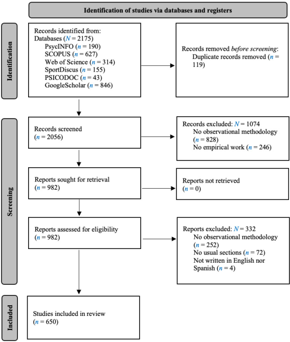
Following PRISMA recommendations (Page et al., 2021), the inclusion criteria for the units of analysis (articles) in this study were as follows. All publications a) relied on observational methodology; b) were empirical; c) presented the usual sections of such studies, e.g., introduction, method, results, and discussion; and d) were written in English or Spanish.
The paper selection was based on an exhaustive search in PsycINFO, SCOPUS, Web of Science, SportDiscus, PSICODOC and Google Scholar to search title, abstract, keywords and full text for the term “observational methodology,” with December 1, 2022, as the cut-off date. The reference list from the articles collected in this step were also examined to identify additional studies.
Instruments
Primary papers included were coded using the MQCOM (Chacón-Moscoso et al., 2019), which assesses the methodological quality in observational methodology studies. It presented validity evidence based on the content of the items and adequate intercoder reliability (> .75). The MQCOM is comprised of 16 rating scale items. Each item receives a score for methodological quality levels of 0 (low), .5 (medium), or 1 (high). Exceptionally, item 11 (Data analysis) had four possible scores (from the lowest to the highest methodological quality level, 0, .33, .67 and 1). This item had a different response scale than the others because it was based on a previous checklist with a rigorous content validity and intercoder reliability study where experts highly recommended increasing the graduation of this item (Chacón-Moscoso et al., 2019). Nonetheless, this item maintains the monotonic incremental function of all ordinal items of the scale, with a range of 0-1 prior to the statistical analysis. The coding manual is available at https://osf.io/uv7cj.
Procedure
Mendeley Reference Manager was used for the search for papers to organize and handle the information obtained through the literature search. During the first screening, the inclusion criteria were applied to the title, keywords, and abstract. The resulting studies were assessed in a second stage in which the inclusion criteria were applied to the full texts. Two coders (DLA and IFM) applied the criteria independently. In case of disagreements, a third coder (SCM) mediated until an agreement was reached.
For the data extraction, IFM and DLA were trained to apply the MQCOM. Each item and its response options were explained. MTA mediated if the explanations differed. Then both coders independently applied the scale to two observational methodology papers to compare the coding. In case of disagreements, a third coder (SSC) mediated. After the training, the coders applied the scale independently to a randomly selected 25% of the sample. Finally, once a high level of consensus was achieved (> .7), DLA applied the scale to the full sample. The data extraction database is available at https://osf.io/m6pvh .
Data Analysis
Using SPSS 27.0, the Intraclass Correlation Coefficient (ICC) was calculated to evaluate both inter and intracoder concordance. Values higher than .7 were considered indicators of adequate reliability (Portney & Watkins, 2000). Additionally, descriptive statistics were provided.
A parallel analysis was then conducted using FACTOR 12 (Ferrando & Lorenzo-Seva, 2017) to obtain empirical evidence of dimensionality. Values higher than .95 for Unidimensional Congruence (UniCo) and higher than .85 for Explained Common Variance (ECV) suggests that data can be treated as essentially unidimensional (Ferrando & Lorenzo-Seva, 2018).
After the parallel analysis, the database was randomly split into two subsamples of 325 papers. With one of the subsamples, an exploratory factor analysis was carried out using SPSS 27.0. First, a polychoric correlation matrix was created with all the variables included in the analysis. Following this step, the statistical assumptions of the matrix were checked by running Bartlett’s test of sphericity, where significant results were considered acceptable, and the Kaiser-Meyer-Olkin (KMO) test, where values higher than .5 were considered adequate (Bartlett, 1954; Kaiser & Rice, 1974). Finally, the exploratory factor analysis was done using principal axis method of factor extraction and Kaiser’s varimax criterion for orthogonal rotation (Field, 2018).
After the exploratory factor analysis, a confirmatory factor analysis was carried out with the second subsample. SPSS 27.0 was used to calculate the internal consistency of the test and the average discrimination index. The internal consistency of the items was measured using Cronbach’s α, where values higher than .7 were considered appropriate. For the average discrimination index, values higher than .4 were considered excellent, .3 - .39 good, and .2 - .29 acceptable (Barbero-García et al., 2015).
The bivariate normality assumption was checked with PRELIS 12 to confirm the suitability of polychoric correlations (Holgado-Tello et al., 2010). The chi-square test (χ2) was run between each pair of correlations assuming a 95% confidence interval with Bonferroni correction α/c (95% confidence level α = .05, and number of contrasts c = [number of items x number of items - 1]/2). The percentage of acceptance of the bivariate normality assumption was then calculated. Additionally, to overcome the large sample size bias in the chi-square test, the Root Mean Square Error of Approximation (RMSEA) was calculated for each pair of correlations, along with the percentage of occasions in which RMSEA was lower than 0.1, the adequate value for parameter estimation (Hooper et al., 2008).
To assess the factor structure of the scale, LISREL 12 was used to estimate the polychoric correlations and the asymptotic variance-covariance matrix. Standardized factor loadings were then calculated (where lambdas of .3 or higher were considered adequate) along with fit indexes (Holgado-Tello et al., 2019; Sanduvete-Chaves et al., 2018), i.e., χ2 (non-significant values -p > .05- allows the null hypothesis of model fit to be accepted, though large sample sizes tend to bias this index towards significant values). Other fit indexes calculated included the Root Mean Square Residual (RMR), where values below .05 were considered adequate); the Root Mean Square Error of Approximation (RMSEA), where values of .08 or lower were considered adequate; the Expected Cross Validation Index (ECVI), where values closer to the saturated model as opposed to the independent model were considered adequate; Critical N (CN), where values higher than 200 were considered adequate; the Parsimony Goodness-of-Fit Index (PGFI), where values between .5 - .9 were considered adequate. Finally, in the following indexes, values higher than .9 were considered adequate: the Normed Fit Index (NFI), the Comparative Fit Index (CFI), the Non-Normed Fit Index (NNFI), the Incremental Fit Index (IFI), the Relative Fit Index (RFI), the Goodness-of-Fit Index (GFI), and the Adjusted Goodness-of-Fit Index (AGFI).
Using JASP version 0.16, the reliability of each factor obtained was studied by calculating McDonald’s Omega (ω). Results higher than .80 were considered strong reliability evidence and .65 - .80, acceptable (Kalkbrenner, 2023). For item discrimination, corrected item-total correlation coefficients were computed. Results were interpreted as excellent when values were higher than .40, good for values between .30 - .40, adequate for .20 - .30, and inadequate for < .20 (Barbero-García, 1993).
Results
Selection of Studies
Figure 1 summarizes the selection process of the papers for this study. The final sample of primary papers included in the study was 650.
Inter and Intracoder Reliability and Descriptive Statistics of the Items
Table 1 presents both inter and intracoder reliability. ICC coefficients were adequate, ranging from .73 to 1.
Table 1. Inter-Intracoder Reliability and Descriptive Statistics of the Items.
| Item | Intercoder Reliability | Intracoder Reliability | Descriptive Statistics | |||||||||
|---|---|---|---|---|---|---|---|---|---|---|---|---|
| ICC | LL | UL | ICC | LL | UL | M | Mdn | SD | S | K | KS | |
| 1 Direct/Indirect | .945 | .926 | .959 | .725 | .495 | .855 | .78 | 1 | 0.38 | -1.33 | 0.09 | .44 |
| 2 Observation Unit | .953 | .936 | .965 | .922 | .854 | .958 | .46 | .5 | 0.45 | 0.15 | -1.75 | .29 |
| 3 Temporality | .947 | .928 | .961 | .976 | .955 | .987 | .46 | .5 | 0.45 | 0.17 | -1.73 | .29 |
| 4 Dimensionality | .933 | .910 | .950 | .845 | .712 | .917 | .47 | .5 | 0.46 | 0.14 | -1.79 | .30 |
| 5 Codification manual | .967 | .955 | .975 | .877 | .771 | .934 | .77 | 1 | 0.35 | -1.16 | -0.02 | .40 |
| 6 Data type | .957 | .942 | .968 | .835 | .692 | .912 | .63 | .5 | 0.33 | -0.32 | -0.75 | .28 |
| 7 Observation instrument | .958 | .944 | .969 | .904 | .822 | .949 | .72 | 1 | 0.42 | -0.95 | -0.90 | .41 |
| 8 Software | .797 | .733 | .846 | .871 | .759 | .931 | .13 | 0 | 0.33 | 2.14 | 2.70 | .51 |
| 9 Type of parameter | .961 | .947 | .971 | .858 | .736 | .924 | .65 | .5 | 0.29 | -0.14 | -0.58 | .34 |
| 10 Data quality control | .975 | .966 | .982 | .963 | .930 | .980 | .82 | 1 | 0.38 | -1.69 | 0.91 | .50 |
| 11 Data analysis | .988 | .984 | .991 | .920 | .852 | .957 | .95 | 1 | 0.17 | -3.84 | 15.34 | .51 |
| 12 Study objective | .866 | .821 | .899 | .951 | .949 | .953 | .65 | .5 | 0.25 | 0.38 | -0.71 | .41 |
| 13 Theoretical framework | .990 | .986 | .992 | .756 | .747 | .765 | .98 | 1 | 0.11 | -6.19 | 41 | .53 |
| 14 Units of study | .855 | .807 | .891 | 1 | 1 | 1 | .64 | .5 | 0.24 | 0.50 | -0.72 | .42 |
| 15 Sessions | .926 | .900 | .945 | .993 | .987 | .996 | .53 | .5 | 0.46 | -0.13 | -1.79 | .30 |
| 16 Discussion | .945 | .926 | .959 | 1 | 1 | 1 | .66 | .5 | 0.27 | 0.02 | -0.70 | .36 |
Note.ICC = IntraClass Correlation; LL = Lower Limit; UL = Upper Limit; S = skewness; K = kurtosis; KS = Kolmogorov-Smirnov normality test statistic. All ICC and KS statistics yielded p < .05.
Table 1 also presents descriptive statistics. The median was .5 for most of the items, with 0 applying only to item 8 (Software). The means were between .13 and .98, the standard deviations ranged between .11 and .46, and there was no normal distribution of the items.
For items 11 (Data analysis) and 13 (Theoretical framework), means were over .9, which implies a low discrimination capacity. Items 11 (Data analysis), 12 (Objectives), 13 (Theoretical framework) and 14 (Units of study) showed standard deviation of 0.25 or below, which implies a low variability. Items 11 (Data analysis) and 13 (Theoretical framework) also showed an extreme negative skewness (over 3 points). Finally, item 11 (Data analysis) showed an extreme positive kurtosis.
To analyze the relationship between items, polychoric correlations were calculated. Table 2 presents the bivariate polychoric correlation matrix.
Table 2. Polychoric Correlation Matrix.
| Item | 1 | 2 | 3 | 4 | 5 | 6 | 7 | 8 | 9 | 10 | 11 | 12 | 13 | 14 | 15 | 16 |
|---|---|---|---|---|---|---|---|---|---|---|---|---|---|---|---|---|
| 1 Direct/Indirect | 1 | |||||||||||||||
| 2 Observation Unit | .84 | 1 | ||||||||||||||
| 3 Temporality | .82 | 1 | 1 | |||||||||||||
| 4 Dimensionality | .83 | .99 | .98 | 1 | ||||||||||||
| 5 Codification manual | .36 | .29 | .26 | .32 | 1 | |||||||||||
| 6 Data type | .63 | .66 | .64 | .63 | .31 | 1 | ||||||||||
| 7 Observation Instrument | .61 | .60 | .58 | .61 | .52 | .51 | 1 | |||||||||
| 8 Software | .38 | .58 | .59 | .53 | .22 | .52 | .56 | 1 | ||||||||
| 9 Type of parameter | .42 | .55 | .53 | .53 | .32 | .46 | .45 | .38 | 1 | |||||||
| 10 Data quality control | .67 | .44 | .44 | .39 | .39 | .54 | .44 | .42 | .49 | 1 | ||||||
| 11 Data analysis | .40 | .36 | .36 | .30 | .27 | .52 | .24 | .44 | .74 | .65 | 1 | |||||
| 12 Study objective | .20 | .10 | .09 | .09 | .27 | .17 | .05 | .07 | .01 | .10 | .24 | 1 | ||||
| 13 Theoretical framework | .04 | -.05 | -.01 | .11 | -.03 | .09 | .10 | -.13 | -.12 | -.11 | -.16 | .18 | 1 | |||
| 14 Units of study | .13 | .23 | .23 | .23 | -.01 | .04 | .10 | .06 | .06 | .10 | .04 | .18 | .09 | 1 | ||
| 15 Sessions | .21 | .08 | .06 | .06 | .07 | .08 | .13 | .16 | .13 | .21 | .20 | .16 | .06 | .03 | 1 | |
| 16 Discussion | .05 | .04 | .01 | .05 | .16 | -.04 | .01 | -.29 | .04 | .23 | .23 | .14 | -.25 | .05 | -.01 | 1 |
Items 12 (Objectives), 13 (Theoretical framework), 14 (Units of study), 15 (Sessions) and 16 (Discussion section) stood out from the other items since their correlations were negative and/or low (r = -.29 - .23). The highest positive bivariate correlations were between items 2 (Observation unit criteria), 3 (Temporal criteria), and 4 (Dimensionality criteria) (r = .98 - 1), but this triad also correlated with item 1 (Direct/indirect observation) (r = .82 - .84).
Study of Dimensionality
To obtain empirical evidence about the number of factors that the scale presented, a parallel analysis was done. Table 3 presents the result of this analysis.
Table 3. Parallel Analysis.
| F | Real data % of variance | Mean of random % of variance | 95 P of random % of variance |
|---|---|---|---|
| 1 | 42.97 | 13.28 | 15.61 |
| 2 | 10.32 | 11.38 | 12.95 |
| 3 | 8.87 | 10.44 | 11.73 |
| 4 | 7.21 | 9.68 | 10.85 |
| 5 | 6.15 | 8.91 | 9.86 |
| 6 | 6.08 | 8.21 | 9 |
| 7 | 4.41 | 7.5 | 8.19 |
| 8 | 3.4 | 6.82 | 7.47 |
| 9 | 3.06 | 6.11 | 6.78 |
| 10 | 2.03 | 5.39 | 6.07 |
| 11 | 1.85 | 4.63 | 5.51 |
| 12 | 1.58 | 3.87 | 5.02 |
| 13 | 1.44 | 3.06 | 4.55 |
| 14 | 0.6 | 2.26 | 3.93 |
| 15 | 0.02 | 1.26 | 2.87 |
Note. F = factors; P = percentile
Both the percentage of variance and the value of McDonald’s Omega (ω = .87) suggest only one factor to be considered. Nevertheless, the UniCo = .41 and the ECV = .31 lead data to be treated as essentially multidimensional (Ferrando & Lorenzo-Seva, 2018).
Exploratory Factor Analysis
To study the factor structure of the scale, a principal-axis factor analysis with oblimin rotation was conducted on the 16 items. Bartlett’s test of sphericity and the KMO measure verified the sampling adequacy for the analysis, Χ 2 = 0.839, p < .001, KMO = .84, and all the KMO values for individual items were above the acceptable limit of .5 (Field, 2018; Kaiser & Rice, 1974). According to the initial analysis of eigenvalues for each factor in the data, five factors had eigenvalues over 1 and, in combination, these explained 62.23% of the variance. Based on the point of maximum curvature obtained in the scree plot (see Figure 2), two factors that jointly explained 40.81% of the variance were retained.
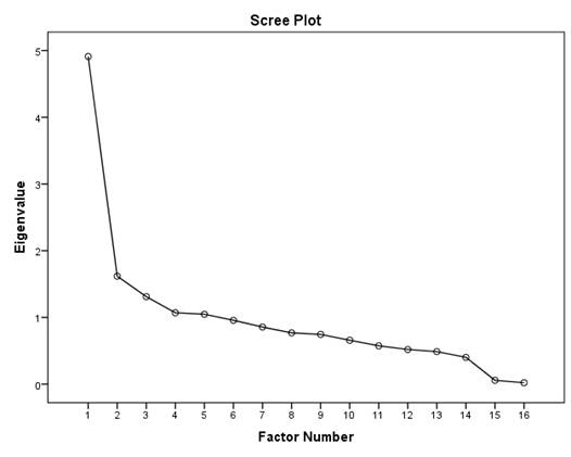
Table 4 presents the rotated factor loadings matrix. As expected, based on the examination of the polychoric correlation matrix (Table 2), items 1 (Direct/Indirect observation), 2 (Observation unit criteria), 3 (Temporal criteria), and 4 (Dimensional criteria) presented high correlations and showed high loading values in the same factor. Items 6 (Data type), 7 (Observation instrument), and 9 (Type of parameters) showed similar loadings in both factors. On the other hand, cut-off point for factor loading was set at .3. Items 12 (Study objective), 13 (Theoretical framework), 14 (Observation units), 15 (Sessions), and 16 (Discussion), all of which had negative and/or low correlations with all other items, presented factor loadings below .3 for both factors and were excluded from the study.
Table 4. Rotated Factor Loadings Matrix Set to Two Factors.
| Item | F1 | F2 |
|---|---|---|
| 1 Direct/Indirect | .54 | |
| 2 Observation Unit | .97 | |
| 3 Temporality | .97 | |
| 4 Dimensionality | .94 | |
| 5 Codification manual | .53 | .48 |
| 6 Data type | .41 | |
| 7 Observation Instrument | .45 | |
| 8 Software | .52 | .53 |
| 9 Type of parameter | .54 | .56 |
| 10 Data quality control | .34 | .62 |
| 11 Data analysis | .52 | |
| 12 Study objective | ||
| 13 Theoretical framework | ||
| 14 Units of study | ||
| 15 Sessions | ||
| 16 Discussion |
Note.F = factor. We only present values higher than the cut-off point for factor loading, set at .3.
The items that cluster on factor 1 were items 1 (direct/indirect observation), 2 (unit criterion of the observational design), 3 (temporal criterion of the observational design), 4 (dimensional criterion of the observational design), 5 (codification manual), and 6 (data type), suggesting that factor 1 represents the quality of the study design. The items that cluster on factor 2 were items 7 (observational instrument), 8 (software), 9 (type of parameter), 10 (data quality control), and 11 (data analysis), suggesting that factor 2 represents the quality of the measurement and analysis.
Confirmatory Factor Analysis
Based on the results of the parallel analysis, it was determined that a single factor should be retained, and that data should be treated as essentially multidimensional. This, in addition to the similar factor loadings that several items displayed in both factors, led to a decision to carry out a second-order confirmatory factor analysis.
Internal Consistency
Internal consistency was good, ω = .87. Factors produced values higher than .6, which was considered appropriate, ωF1 = .90; ωF2 = .68.
Average Discrimination Index
The global average discrimination index (D) was considered appropriate at .55. Factors also produced appropriate values, DF1 = .46, DF2 = .67.
Bivariate Normality Assumption
Data produced a matrix of 55 pairs of items ([11 x 10]/2). The bivariate normality assumption was accepted in 63.6% of occasions (35 correlations), pcorrected = .05/55 = .0009. Additionally, RMSEA values were below 0.1 72.7% of the time (40 correlations), so the factor analysis can be based on polychoric matrix.
Model Fit
The χ2 test was significant χ2 (42) = 531.79, p < .001, probably due to the sensitivity of this test to high sample sizes. RMR was 0.084, yielding a result slightly higher than expected. The other indexes showed an appropriate fit on the second-order factor model, RMSEA = 0.000, 90% CI [0.000, 0.000]; ECVI = 0.28 (saturated ECVI = 0.41; independent ECVI = 16.37); CN = 37964663941.58; PGFI = .62; NFI = 1; CFI = 1; NNFI = 1.01; IFI = 1.01; RFI = 1; GFI = .98; AGFI = .97.
Therefore, it seems logical to accept a factor structure comprised of a quality design factor and a quality measurement and analysis factor, both grouped under a second-order global methodological quality factor. Figure 3 shows the MQSOM structure with the standardized factor loadings.
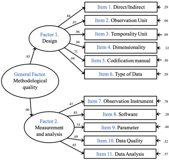
Figure 3. Structure of the Methodological Quality Scale for Observational Methodology Studies with the Standardized Factor Loadings.
Table 5 shows the descriptive statistics for each factor. Reliability yielded strong-acceptable evidence, and discrimination was excellent.
Table 5. Descriptive Statistics of the Factors.
| First Order Factors | Second Order Factor | ||
|---|---|---|---|
| Descriptive statistic | Factor 1 Design quality | Factor 2 Measurement and analysis quality | General Factor (Methodological quality) |
| Mean | 0.51 | 0.76 | 0.62 |
| Standard deviation | 0.32 | 0.21 | 0.24 |
| McDonald's Omega | .9 | .68 | .87 |
| Average discrimination | .46 | .67 | .55 |
Note.Mean and standard deviation values range from 0 to 1.
Interpretation of the Study Scores
Factor 1 (F1) assesses the quality of the design and is formed by item 1 (observational methodology mentioned), item 2 (observation unit criteria mentioned), item 3 (temporal criteria mentioned), item 4 (dimensionality criteria mentioned), item 6 (codification manual defined), and item 8 (data type specification mentioned). The research design of studies with high F1 scores would be based on the existing literature on observational methodology, with an explicit delimitation of its observational design, as well as the data type and the manual that supported the subsequent observation process. Factor 2 (F2) assesses the quality of the measurement and the analysis, and it is formed by item 5 (observation instrument adequacy), item 7 (software used), item 9 (type of parameter considered), item 10 (type of data quality control), and item 11 (type of data analysis performed). Studies with high F2 scores would be characterized by robust observational methodology research procedures, capable of drawing well-defined results based on a detailed methodology that leads to reliable conclusions. Finally, a global second-order factor (GF) of methodological quality encompasses the quality of both the design and of the measurement and analysis.
Item scores ranged from 0 to 1, as did the averages of the first and second order factors. Values below .5 were considered low, values between .5 and .75 (both values included) were considered medium, and values over .75 were considered high. Table 6 shows an example of the interpretation of the methodological quality of a set of studies based on the scores for each item and the subsequent mean per factor.
Table 6. Scores of Each Item from Five Studies and Average Values for Each Factor.
| Studies | Factor 1 | Factor 2 | Average | |||||||||||
|---|---|---|---|---|---|---|---|---|---|---|---|---|---|---|
| I1 | I2 | I3 | I4 | I5 | I6 | I7 | I8 | I9 | I10 | I11 | F1 | F2 | GF | |
| Serna et al. (2017) | 1 | 1 | 1 | 1 | 1 | 0 | 1 | .5 | 1 | 1 | 1 | .83 | .90 | .87 |
| Lappi et al. (2017) | 0 | 0 | 0 | 0 | 0 | 0 | 0 | .5 | 0 | 0 | 0 | 0 | .10 | .05 |
| Lapresa et al. (2017) | 1 | 1 | 1 | 1 | 1 | 1 | 1 | 1 | 1 | 1 | 1 | 1 | 1 | 1 |
| Maciá et al. (2021) | 1 | 0 | 0 | 0 | 1 | 0 | 1 | .5 | .5 | 1 | 1 | .33 | .80 | .57 |
| Argudo-Iturriaga et al. (2021) | 1 | 0 | 0 | 0 | 1 | 0 | .5 | .5 | .5 | 1 | 1 | .33 | .70 | .52 |
Note.I = item; F1 (first order factor 1) = Design; F2 (first order factor 2) = Measurement and analysis; GF (second order general factor) = Methodological quality. Interpretation for each factor: < 0.5 - Low quality level, 0.5 - 0.75 - Medium, > 0.75 - High quality level.
Table 7 presents the frequency and percentage of studies analyzed that fell into each level of quality for F1, F2, and the GF. The quality levels of most of the studies included were considered low in terms of the design (47.8%) and high in terms of the measurement and analysis (61.8%). In terms of overall methodological quality, the sample is distributed fairly equally between the quality levels, with a slight predominance of the high level of methodological quality (36.8%).
Table 7. Distribution of the Sample by Quality Level.
| Quality level | F1 Quality of the Design | F2 Quality of the Measurement and Analysis | GF Methodological Quality |
|---|---|---|---|
| Low | 311 (47.8) | 70 (10.8) | 203 (31.2) |
| Medium | 133 (20.5) | 178 (27.4) | 208 (32.0) |
| High | 206 (31.7) | 402 (61.8) | 239 (36.8) |
| Total | 650 (100) | 650 (100) | 650 (100) |
Note.Percentages are presented in brackets. Interpretation for each factor: < 0.5 - Low quality level, 0.5 - 0.75 - Medium, > 0.75 - High quality level.
Finally, Table 8 presents the resulting MQSOM tool to measure the methodological quality in observational methodology studies.
Table 8. Methodological Quality Scale for Observational Methodology Studies.
| Factor 1. Quality of the Design | |
|---|---|
| Item 1 | Direct/indirect observation: Reference to observational methodology, specifying whether observation is direct or indirect: 0: Methodology is not referenced. 0.5: Yes, justified but not documented. 1: Yes, justified and documented. |
| Item 2 | Observation unit criteria (idiographic: study units are formed by one or more participants if there is a stable link between them; nomothetic: two or more study units): 0: Not identified. 0.5: Yes, observation units are identified, but without justification.1: Yes, observation units are identified, with justification for the choice of an idiographic or nomothetic approach in accordance with the study objectives. |
| Item 3 | Temporal criteria (punctual: one or two observation sessions; follow-up: more than two observation sessions): 0: Not identified. 0.5:: Criterion of temporality identified, but without differentiating. 1: Temporality criterion identified, differentiating between-session and within-session follow-up. |
| Item 4 | Dimensionality criteria (one-dimensional: one level of response; multidimensional: two or more levels of response): 0: Not identified. 0.5: Dimensions identified without reference to any conceptual framework. 1: Dimensions identified based on a conceptual framework. |
| Item 5 | Codification manual with definition of the categories/behaviors and specification of dimensions (in multidimensional designs): 0: Manual not available. 0.5: Partial information (e.g., dimensions specified, but without definition of the categories/codes of each dimension). 1: Codification manual with definition of the categories/behaviors and specification of dimensions (in multidimensional designs). |
| Item 6 | Specification of data type (I, II, III, and IV [Bakeman, 1978]) as sequential/concurrent (sequential data: behaviors that cannot overlap and belong to a single dimension; concurrent data: behaviors that can co-occur and belong to several dimensions) and event-based/time-based (event-based: the primary parameter used in the record is order of events; time-based: the primary parameter is duration): 0: Data type not specified. 0.5: Data type specified but not justified. 1: Data type specified with justification. |
| Total factor 1 | Quality of the Design score: Add the scores obtained in items 1-6 and divide by the number of items. |
| Factor 2. Quality of the Measurement and Analysis | |
| Item 7 | Adequacy of the observation instrument (combination of field format with category system, field format, category system, or scale of estimation [Anguera, 2003]): 0: Observation instrument not available (e.g., only a list of behaviors provided). 0.5: Observation instrument described but not justified based on the objectives and observational design. 1: Observation instrument justified according to the objectives and observational design. |
| Item 8 | Software used to register data (SDIS-GSEQ v. 4.2.1./GSEQ 5, LINCE, MATCH VISION STUDIO, Transana, other: specify), control data quality (SDIS-GSEQ v. 4.2.1./GSEQ 5, LINCE, HOISAN, GT, SAS, other: specify), and analyze data (SDIS-GSEQ, HOISAN, THEME v. 6, R, SAS, other: specify): 0: Not used. 0.5: Used partially, only for some of the three aspects. 1: Used to register data, control data quality, and analyze data. |
| Item 9 | Type of parameters according to given use (Bakeman, 1978): 0: Primary, or basic, registration of a single category: frequency, order, and duration. 0.5: Secondary, derived from a single category record (ratios between primary indicators): average frequency, relative frequency, rate, relative duration, average duration, and other: specify. 1: Mixes, dynamic, or transition (two categories considered to analyze the transition from one category to another): transition frequency, relative frequency of transition, and relative duration of transition. |
| Item 10 | Between-observer reliabilityz (agreement between the records of different observers)/within-observer reliability (agreement between the records of the same observer at two time points): 0: Not assessed. 0.5: Consensual agreement (qualitative). 1: Agreement is global (based on primary indicators, frequency, and duration) sequential (based on sequential-order indicators: Pearson correlation, Berk intra-class coefficient, etc.); or point-by-point (each record that each observer registers is compared): e.g., total percentage of agreement, kappa coefficient, generalizability theory). |
| Item 11 | Type of data analysis performed (Blanco-Villaseñor et al., 2003): 0: No data analysis. 0.33: Qualitative analysis only. 0.66: Descriptive analysis only. 1: Inferential analysis: relationship between categorical data (comparison of proportions); analysis of regularities (sequential analysis of delays, Markov chains, T-pattern detection, analysis of polar coordinate); multivariate analysis (logistic regression, log-linear, logit-probit, correspondence analysis); analysis of the temporal dimension (panel studies, trend analysis, time series); nonparametric tests; tests of relation (ordinal correlation, linear correlation, multiple correlation); multidimensional scaling; other: specify. |
| Total factor 2 | Quality of the Measurement and Analysis score: Add the scores obtained in items 7-11 and divide by the number of items. |
| Global factor | Methodological quality score: Add the scores obtained in factors 1 and 2 and divide by 2. |
Note.Interpretation for each factor: < 0.5 - Low quality level, - Medium, > 0.75 - High quality level.
Discussion
This study obtained a simple and useful scale comprised of 11 items to measure methodological quality in many professional areas where observational research is conducted. The Methodological Quality Scale for Observational Methodology studies (MQSOM) includes a second-order methodological quality factor that contains two first-order factors; these serve as indicators of quality of both the design and of the measurement and analysis.
By creating the first scale to measure methodological quality in studies based on observational methodology, this work responds to one of the most important needs in a promising and fruitful area of the behavioral sciences. The main strength of this scale is that it is based on results obtained over the last 30 years by our research group and relies on a broad review of 650 observational methodology studies.
One possible limitation of this study is the lack of unpublished studies on observational methodology. Although the paper selection process did not need to be exhaustive, experts could have been consulted to obtain this kind of grey literature to strength the sample that formed the basis for the MQSOM (Sánchez-Meca, 2022). For further research, validity evidence of MQSOM will be explored based on its convergence and divergence with other instruments applied in mixed method research. Also, a guide will be drafted to inform applied researchers across a wide range of disciplines about the quality of design, measure and analysis, and methodological quality as an overall assessment of intervention programs based on observation (Muñiz & Fonseca-Pedrero, 2019).
This original contribution can be considered a milestone in the development of a methodological culture based on systematic observation. The MQSOM serves as both an assessment tool and as a guide. Thus, it should be disseminated among researchers in the years to come in order to first help authors to assess the methodological quality of their observational methodology studies and also guide applied researchers in the design and implementation of intervention programs based on observational methodology. Furthermore, this scale could become a reference for editorial boards and other decision-making committees. Readers and potential users are encouraged to share their results when applying the scale, to strengthen its potential.

