The exploratory factor analysis of items: guided analysis based on empirical data and software

El análisis factorial exploratorio de los ítems: análisis guiado según los datos empíricos y el software

 

 

Susana Lloret, Adoración Ferreres, Ana Hernández and Inés Tomás

Behavioral Scinces Methodology Department and IDOCAL Research Institute. Universitat de Valencia (Spain)

Correspondence

 

 

---

ABSTRACT

The aim of the present study is to illustrate how the appropriate or inappropriate application of exploratory factor analysis (EFA) can lead to quite different conclusions. To reach this goal, we evaluated the degree to which four different programs used to perform an EFA, specifically SPSS, FACTOR, PRELIS and MPlus, allow or limit the application of the currently recommended standards. In addition, we analyze and compare the results offered by the four programs when factor analyzing empirical data from scales that fit the assumptions of the classic linear EFA modeling adequately, ambiguously, or optimally, depending on the case, through the possibilities the different programs offer. The results of the comparison show the consequences of choosing one program or another; and the consequences of selecting some options or others within the same program, depending on the nature of the data. Finally, the study offers practical recommendations for applied researchers with a methodological orientation.

Key words: Exploratory Factor Analysis; SPSS; FACTOR; PRELIS; MPlus.

---

RESUMEN

El objetivo del presente trabajo es ilustrar cómo la aplicación adecuada o inadecuada del análisis factorial exploratorio (AFE) puede llevar a conclusiones muy diferentes. Para ello se evalúa el grado en que cuatro paquetes estadísticos diferentes que permiten realizar AFE de ítems, en concreto SPSS, FACTOR, PRELIS y MPlus, permiten o limitan la aplicación de los estándares actualmente recomendados en materia de análisis factorial. Asimismo se analizan y comparan los resultados que ofrecen dichos programas cuando se factorizan datos empíricos de escalas que ajustan, según el caso, de manera inadecuada, ambigua u óptima a los supuestos del modelo AFE lineal clásico, a través de las distintas posibilidades que ofrecen los distintos programas. Los resultados de la comparación ilustran las consecuencias de elegir entre un programa u otro, y también las consecuencias de elegir entre unas opciones u otras dentro de un mismo programa, en función de la naturaleza de los datos. Finalmente se ofrecen una serie de recomendaciones prácticas dirigidas a los investigadores aplicados con cierta orientación metodológica.

Palabras clave: Análisis Factorial Exploratorio; SPSS; FACTOR; PRELIS; MPlus.

---

 

Introduction

This article is the continuation of "Exploratory factor analysis of items: a revised and updated practical guide" (Lloret, Ferreres, Hernández, & Tomás, 2014), published in this journal. That article and the following one "Exploratory factor analysis of items: some additional considerations" (Ferrando & Lorenzo-Seva, 2014) present the currently recommended standards for the applied researcher in terms of factor analysis (FA). In this second part, first we will review and summarize the degree to which four different statistical packages, SPSS version 22.0, FACTOR version 10.3.01 (Lorenzo-Seva & Ferrando, 2006, 2013), PRELIS¹ version 9.10 (Jöreskog & Sörbom, 2007) and MPlus version 6.12 (Muthén & Muthén, 2007, 1998-2012), allow or limit the application of these standards. Second, we will analyze the results offered by each of these programs when factor analyzing empirical data from scales that inadequately, ambiguously, or optimally fit, depending on the case, the assumptions of the exploratory factor analysis (EFA) classic linear model. These three practical cases with real data will allow us to compare the consequences of choosing a particular software; and the consequences of selecting the different options within the same software, when the data are more or less "problematic". Our objective is clear: to illustrate how the appropriate or inappropriate application of EFA can lead to very different conclusions.

SPSS, FACTOR, PRELIS, and Mplus vary in the degree to which they allow the application of current standards. Following the brief guide we presented in the first part (Lloret et al., 2014), it would be desirable for these programs to offer all the options included in Table 1, or at least most of them. However, not all of them do so.

 

 

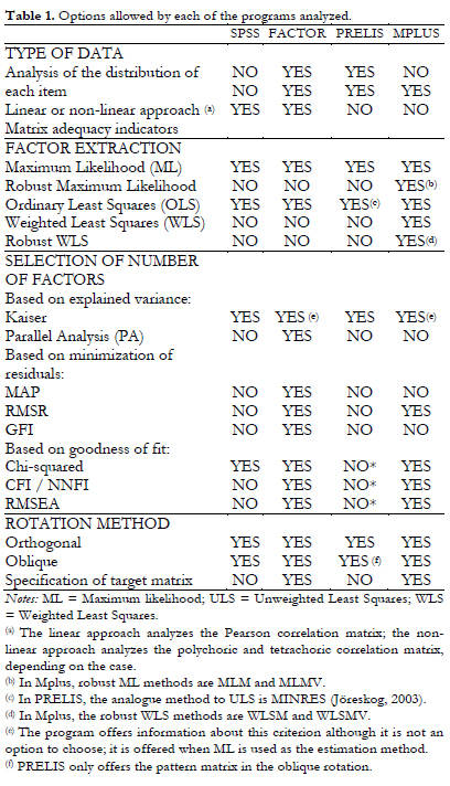
The information included in Table 1 shows that the most complete program is FACTOR, the only one specifically designed for FA, and a freeware program. It only lacks a factor extraction method such as weighted least squares, and its authors are already working on this (Ferrando & Lorenzo-Seva, 2014). The strength of Mplus lies in the factor extraction methods. However, it leaves out a basic aspect, which is the evaluation of the adequacy of the matrix for factorization, and the researcher is limited by the factor selection criteria Mplus offers. PRELIS limits the researcher even more because it does not allow the user to determine the number of factors to be extracted: it does this automatically by applying the Kaiser criterion (Kaiser, 1958). Finally, a limitation imposed by SPSS is that it only allows the analysis of the items using the linear approach, although this aspect can be mitigated to a certain extent by the use of the free non commercial SPSS programs TETRA-COM and POLYMAT-C (see, Lorenzo-Seva & Ferrando, 2012, 2015). For more information, consult the Annex, which offers a summary of the possibilities and limitations of SPSS, FACTOR, PRELIS and MPlus.

Taking into account the current standards recommended for performing EFA (Ferrando & Lorenzo-Seva, 2014; Lloret et al., 2014) and the options of the different programs (whose main characteristics and strong and weak points are described in the Annex), various recommended roadmaps can be offered for each program. We hope these results are useful for the applied researcher. The recommended road map for the SPSS program is the following: 1) items that show average difficulty and discrimination levels, have a sufficient number of response categories (minimum 5), and present approximately normal distributions; 2) are analyzed by means of Maximum Likelihood (ML), or Unweighted Least Squares (ULS) estimation methods (knowing that ML provides "reliable" indicators of the goodness of fit of the model, although at times non-convergence estimation problems or Heywood² cases can appear, whereas ULS is more robust in the estimations (specially on complex solutions) but less robust in the assessment of goodness of fit); 3) combining different factor selection criteria (Kaiser, scree-test, explained variance, and baseline theory); and 4) opting for an oblique rotation method such as PROMAX or OBLIMIN. Nevertheless, researchers must be aware that if the default options of SPSS are used (the famous "Little Jiffy" combination of Principal Components regardless of the type of items + Kaiser criterion + Varimax rotation), it will be probably used in the worst possible way. Unfortunately, this type of EFA analysis by default is still quite frequent.

For FACTOR, we recommend the following two roadmaps depending on the characteristics of the sample and the data. The first would be the one that: 1) fits the nonlinear model in large samples, when items are dichotomous or polytomous with few graded response categories, and they do not fulfill the condition of average difficulty and discrimination; 2) analyzing the tetrachoric or polychoric correlation matrix; 3) using the ULS estimation method; 4) combining the different factor selection criteria: Parallel Analysis (PA),the Minimum Average Partial (MAP) test, the goodness of fit indices available when using polychoric correlations, residuals minimization, and, finally, the baseline theory; and 5) opting for the PROMIN rotation, flexible but simple. The other possible combination would be the one that: 1) fits the linear model in small or medium samples, when items show average difficulty and discrimination levels (with approximately normal distributions) and have a sufficient number of response categories (minimum 5); 2) analyzing the Pearson correlation matrix; 3) using ML or ULS estimation methods; 4) combining the different factor selection criteria (PA or MAP, residuals minimization, goodness of fit indices, and the baseline theory); and 5) opting for the PROMIN rotation, flexible but simple. The least recommendable option is to fit the non-linear model using the ULS method when samples are small or questionnaires have a large number of items. In these circumstances, this unweighted method offers problematic solutions in the assessment of fit.

For PRELIS, we recommend following one of these two roadmaps, depending on the characteristics of the sample and the data. 1) For small or medium samples, when the linear model is an adequate approximation to the data because the items have a sufficient number of categories (minimum 5) that reasonably fit a normal distribution; 2) the Pearson correlation matrix is factorized; 3) using the ML or MINRES (MINimum RESiduals) estimation method, equivalent to ULS; 4) following the Kaiser criterion, and evaluating the fit of the successive models that can be compared when employing ML³; and 5) the oblique solution is interpreted, which can be compared to the orthogonal solution (both are provided by the program by default). Or 1) for large samples, when the linear model is not appropriate because the items are dichotomous or polytomous with few graded response categories that do not fulfill the condition of average difficulty and discrimination; 2) analyzing the tetrachoric or polychoric correlation matrix; 3) using the MINRES estimation method; 4) employing the Kaiser criterion, as it is the only one offered; and 5) interpreting the oblique solution which can be compared to the orthogonal one.

And in MPlus, the two most appropriate road maps, depending on the characteristics of the sample and the data, would be the following: one that 1) analyzes the non-linear model in large samples and dichotomous or polytomous items with few graded response alternatives that do not fulfill the condition of average difficulty and discrimination; 2) analyzing the tetrachoric or polychoric correlation matrix; 3) using a robust Weighted Least Squares (WLS) estimation method such as WLSMV (see details about the characteristics of the different estimation methods in the Annex); 4) combining the different factor selection criteria (residuals minimization, incremental fit indices, and the baseline theory); and 5) opting for an oblique rotation such as GEOMIN. The second route would be to: 1) analyze the linear model in small and medium samples and items with average difficulty and discrimination and a sufficient number of response categories (minimum 5); 2) analyzing the Pearson correlation matrix; 3) using the ML estimation method, or MLMV if the data do not follow an approximately normal distribution; 4) combining the different factor selection criteria (residuals minimization, incremental fit indices, and the baseline theory); and 5) opting for an oblique rotation, such as GEOMIN.

As would be expected, we cannot generate an algorithm that guides the researcher's decisions through the different options mentioned, but we can summarize the rules to follow. The decision begins with the focus of the analysis: linear or non-linear. This decision is controversial because it involves the two conflicting aspects that characterize a good model: simplicity and realism. These two qualities do not go together: the non-linear model is realistic, and the linear model is simple. It is worth mentioning that the simplest approach is often also the most useful one because it offers better fit (Ferrando & Lorenzo-Seva, 2014). However, no simulation studies have been conducted to make recommendations in this regard, especially in the case of the factor estimation methods (Muthén & Asparouhov, 2010). For the moment, we can say that the optimal situation to apply the linear approach is the one that analyzes a set of ordinal items that are close to the continuity assumption because they have a normal multivariate distribution or normal univariate distributions and five or more response categories (Flora, LaBrish, & Chalmers, 2012). In addition, the linear approach is recommended when analyzing a relatively large set of items in a relatively small sample, provided that the items have approximately normal univariate distributions or, at least, symmetric distributions and average difficulty and discrimination levels, and have five or more response alternatives (Ferrando & Anguiano-Carrasco, 2010; Muthén & Kaplan, 1985). When these conditions are not present, the non-linear approach will be more realistic (Ferrando & Lorenzo-Seva, 2013, 2014). We must remember that it is especially important to consider the relationship between the sample size, number of items, and number of response alternatives per item. If there are a large number of items and/or they have five or more response alternatives, no matter how large the sample is, the estimations of the polychoric/tetrachoric correlations will be unstable. We summarize all of these recommendations in Table 2.

We illustrate the application of the recommended roadmaps for the four aforementioned programs. Specifically we will analyze the factor structure of three sets of scales: the Strength and Flexibility scales of the PSDQ (Physical Self-Description Questionnaire; Marsh, Richards, Johnson, Roche, & Tremayne, 1994); the Self-esteem and Selfconcept scales of the PSDQ (Marsh et al., 1994); and the D-48 test (Anstey, 1959. Adapted by the I+D+I Department of TEA Editions, 1996). We analyzed real responses, with the special circumstance that these responses fit the assumptions of the linear or classic EFA model optimally, ambiguously, or inadequately, depending on the scale (Fabrigar, Wegener, MacCallum, & Strahan, 1999).

 

Method

Sample

We used two incidental samples and analyzed three sets of data. The first dataset selected corresponds to the responses of a sample of 914 subjects on the Strength and Flexibility Scales of the PSDQ. Following the criteria presented in Table 2, this set of data would represent the optimal situation, as they acceptably meet the assumptions of the classic or linear factor analysis because: 1) the items present approximately normal distributions -with skewness and kurtosis less than 1 in absolute values-; 2) there are 6 response alternatives; 3) the sample size is large (n = 914), and in addition, the favorable conditions of having 6 items per factor, and only two factors are observed. Moreover, these two factors present a low correlation with each other.

The second set of data chosen corresponds to the responses of a sample of 976 subjects on the Self-esteem and Physical Self-concept scales of the PSDQ. This dataset offers an ambiguous fit because it only partially meets the assumptions of the classic or linear factor analysis, as: 1) it does not fulfill the condition of average location/difficulty (item means range between 4.04 and 5.11 on a response scale from 1 to 6, and the skewness coefficients of 6 of the 14 items are greater than 1 in absolute value); 2) but the inter-item correlations range between .25 and .73, with 74% being less than .50 (M = .42, SD = .13), which indicates that the condition of moderate discrimination is met; 3) the items are answered with 6 response options; and 4) the sample size is large (n = 976). Moreover, favorable circumstances of having six and eight items, respectively, to measure only two factors, are observed.

The third set of data corresponds to the responses of a sample of 499 subjects on the D-48 Test. This test measures the "G" factor of intelligence through the correct/error responses the subjects give on a set of 44 domino-type items with different levels of difficulty. This dataset does not meet the assumptions of the classic or linear factor analysis at all because: 1) it does not fulfill the average location/difficulty condition (the distributions of the items are strongly skewed, some quite easy and others quite difficult); 2) the items are dichotomous; 3) the sample size is large (n = 499); 4), but the test is long, containing 44 items; and 5) the items measure one factor. Furthermore, there is a collinearity problem between two items (probably due to an item duplicated by mistake: their correlation was 1). When we detected this anomaly, we decided to leave it in, in order to detect how each program responded to it.

The recommendation of the classic or linear factor analysis in the first set of data is clear, as it represents the optimal condition for linear analysis. In the second set of data, the recommendation about the type of analysis is not as clear, although the linear approach, simpler and more robust, is the first option for analysis. Here we have the ambiguous condition. In the third set of data, however, the recommendation is the non-linear approach, as it represents the inadequate condition for the linear model.

Procedure

We analyzed each set of data under various conditions:

1) Only with SPSS, the "Little Jiffy" criterion: Principal Components Analysis (PCA) + Kaiser criterion + VARIMAX rotation (VAX). We included this combination because, in spite of not being a factor analysis, and therefore not one of the recommended options, it is still the most popular combination and the one most frequently utilized, perhaps because it appears by default in SPSS (see, Izquierdo, Olea, & Abad, 2014).

2) With the four programs (SPSS, FACTOR, PRELIS and MPlus), we applied the most appropriate approach considering the options offered by each program and the criteria presented (see, Table 1 and Table 2). In cases where there was more than one adequate approach, or more than one adequate option within the same approach, we started by applying the most advisable combination, and we modified it based on the results obtained.

In a reiterative way and in each case, we evaluated each solution according to two criteria or principles: the Statistical Plausibility principle and the Theoretical Credibility principle. On the one hand, we consider a statistical solution to be plausible when none of the following appears: Convergence problems, non-positive definite matrices, or Heywood cases. These would be indicators that the solution reached, in spite of being statistically possible, is not plausible, but rather forced. On the other hand, we consider that a solution is credible when it offers interpretable results considering the content of the items and the meaning of the factors according to the theory.

 

Results

Strength and Flexibility Scales. Optimal condition for the linear approach

Table 3 shows the set of exploratory factor analyses carried out by means of the four programs under evaluation following the linear approach (i.e. factor analyzing the Pearson correlation matrix). All of these analyses lead to a plausible and credible result that identifies the two expected factors, except the analysis with MPlus (in version 6, used in the present study).

When we apply "Little Jiffy" with SPSS, we obtain similar results to those obtained also through SPSS with the ML + Kaiser + Oblimin combination, and to those obtained through FACTOR with the ML + 2F + Promin combination: 2 well-defined factors⁴. All of the items loaded above .50 on the expected factor and below .30 on the other one. In both programs, SPSS and FACTOR, the selection criteria of the number of factors used in each case lead to the same number that we had previously established: two factors.

In the case of PRELIS (version 9.10), in spite of having a dialogue box with the option to fix the number of factors, the program does not really allow the researcher to do so. Among the examples tested (those from the present study and from others), if we mark the option of retaining a lower number of factors than the number determined by the Kaiser criterion, the output still shows the solution for the number of factors suggested by Kaiser. If a larger number is specified, the program does not print the results, at least among all the examples tested, and it only shows the distributional analyses of the items. The solution is only printed when the number of factors coincides with what is suggested by the Kaiser criterion. In sum, PRELIS automatically applies the Kaiser rule, and in this case, it retains two factors that are well-defined and consistent with what was expected and with the results of SPSS and FACTOR.

By contrast, with MPlus, four factors were selected. The comparison of the sequence of models it estimates (a model with zero factors up to the model with nine factors, the maximum allowed) shows that the fit improves as the number of factors increases. However, from five factors on, the solution no longer converges. The 4-factor model presents the best fit (CFI = .998, NNFI = .993, RMSEA = .025, SRMR = .011), according to the comparative incremental fit indices. However, an analysis of both, the structure matrix and the pattern matrix, shows the presence of two major factors and two minor ones. The six items in the strength factor are grouped in the first factor, whereas five of the six flexibility items are grouped in the second factor. The third factor includes only one item of the flexibility scale, and in factor 4, no item presents factor loadings above .40. The factor solution of the 4-factor model is statistically plausible but in reality not very credible. However, the 2-factor model already presents satisfactory goodness of fit indices (CFI = .960, NNFI⁵ = .939, RMSEA = .077, SRMR = .025), whereas the 1-factor model does not (CFI = .578, NNFI = .484, RMSEA = .224, SRMR = .185). Analyzing both, the structure matrix and the pattern matrix of the 2-factor model, results show well-defined factors, with the expected item groupings.

Finally, it is worth noting that there were no convergence problems or parameter estimates outside their permissible range. In addition, since the model was not complex, we did not consider it necessary to use ULS and we only tested the ML estimation method.

Self-esteem and Self-concept scales. Ambiguous condition for the linear approach

Table 4 shows the set of EFAs that we performed on this set of data. We analyzed the linear and non-linear approaches when the programs allowed it (all of them except SPSS).

When we apply "Little Jiffy" with SPSS, we obtain results similar to those obtained with the ULS + Kaiser + Oblimin combination: Two major factors, a minor factor, and a mixed item. Specifically, the six overall physical selfconcept items are grouped in the first factor, along with an item from the self-esteem scale (ES6) that is mixed. For the mixed item, the factor loadings on the overall physical selfconcept and the self-esteem factors are .55 and .44, respectively, when PC is used, and .50 and .40, respectively, when ULS is used. This tendency of PC to overestimate or at least offer higher factor loadings than the true FA methods has been repeatedly observed throughout the different analyses carried out in the present study and documented in previous studies (e.g. Ferrando & Anguiano-Carrasco, 2010; Izquierdo et al., 2014). On the other hand, six of the eight self-esteem items are grouped in the second factor (including the mixed item). Finally, two other self-esteem items (SE1 and SE5), which are found to be redundant because their wording is quite similar, are grouped in the third factor, with high factor loadings (.81 and .84 with PCA, and .69 and .84 with ULS, for SE1 and SE5, respectively).

Even though the data are not normally distributed, if we use ML with SPSS we would obtain a solution with parameter estimates that are outside their permissible range of values. Specifically, there is a Heywood case (a factor loading of 1.027), so that the solution is not statistically plausible. Although the program does not explicitly refer to this factor loading, it does show the following warning: "one or more communalities greater than 1 have been found during the iterations. The resulting solution should be interpreted with caution". After eliminating mixed item SE6 and one of the redundant items (SE5), the 2-factor model is adequate, although item SE1 (item 1 on the self-esteem scale), which appeared in the minor factor, now presents a marginal factor loading of .35.

FACTOR offers practically the same results using the linear and non-linear approaches: the two expected well-defined factors, although again, SE6 appears as a mixed item. The linear "Pearson + ML + 2F + Promin" combination offers loadings slightly inferior to the analogous "Polychoric + ULS + 2F + Promin" combination. We compared the fit of the 2-factor model from each approach on the criteria available in both cases: GFI and RMSR. GFI is .99 in both approaches and RMSR is slightly better in the linear approach (.046 compared to .048). As Ferrando and Lorenzo-Seva (2014) point out, even in conditions where the non-linear model should fit better, the linear model presents better fit. It must be pointed out that the PA criterion recommends one factor for both, the linear and non-linear approaches; however, when the 1-factor model is tested, GFI and RMSR show inadequate goodness-of-fit, leading to the conclusion that two factors are necessary (which is what the theory indicates). Furthermore, the MAP criterion suggests two factors.

Regarding PRELIS, in the non-linear approach (Polychoric + ULS + Kaiser), three factors are obtained. All of the items on the physical self-concept subscale load on the same factor (with factor loadings between .72 and .86 in the PROMAX solution), but the self-esteem items are split into the other two factors (with factor loadings that range between .35 and .81 in the PROMAX solution). The program also detects that item SE6 is mixed. As occurred with SPSS, by eliminating the mixed item and one of the redundant items (SE5), the 2-factor model becomes adequate, although item SE1, as occurs with SPSS, presents a marginal factor loading equal to .38. When using the available linear approach (Pearson + ML + Kaiser), the program also retains three factors, according to the Kaiser rule. However, a Heywood case is obtained (as the program appropriately indicates), so that we do not continue with the interpretation.

MPlus, with a non-linear approach using the WLSMV robust estimation method, recommended in cases of nonnormality like this one (Polychoric + WLSMV), does not present any problem. The goodness-of-fit improves as the number of factors increases. However, from six factors on, the solution no longer converges. Following the criterion of comparing the incremental fit indices, the 3-factor model (CFI = .987, NNFI = .977, RMSEA = .073, SRMR = .021) should be selected. Model 2 shows an acceptable fit (CFI = .943, NNFI = .919, RMSEA = .136, SRMR = .052). However, the improvement in fit of model 3 compared to model 2 is not trivial (ΔCFI = .044, ΔNNFI = .058, ΔRMSEA = -.063); whereas the 4-factor model presents an irrelevant improvement over the 3-factor model (ΔCFI = .006, ΔNNFI = .007, ΔRMSEA = -.012). The one-factor model presents unacceptable fit indices (CFI = .868, NNFI = .844, RMSEA = .190, SRMR = .096). On the other hand, MPlus, with the linear approach "Pearson + ML", apparently has no convergence problems, as there are no advisory or warning messages. The only messages indicate that from a certain number of factors (6 factors), convergence is not reached in the rotation algorithm, and therefore the 6-factor model or any other model with more than six factors is not estimated. However, two Heywood cases appear which means that those results are not statistically plausible. Thus, we do not interpret this solution, only interpreting the results of the non-linear approach.

The analysis of both the structure matrix and the pattern matrix shows that the results from SPSS and PRELIS are repeated: Two major factors and one minor factor are obtained, as well as a mixed item. Again, the results show that when the mixed item (SE6) and one of the redundant items (SE5) are eliminated, the 2-factor model is the most adequate (CFI = .992, NNFI = .987, RMSEA = .061, SRMR = .021), with the factor loading of item SE1 being marginal (.375).

D-48. G Factor Scale. Inadequate condition for the linear approach

We will recall that this set of data is especially problematic from the point of view of factor analysis: the markedly asymmetric distributions of the items, which are generally quite easy or quite difficult, dichotomous, in a sample that is not large enough for the large number of items, and the duplication of one of the items, makes it quite difficult to successfully analyze the set of items. Table 5 shows the results we obtained.

With SPSS, we obtained the "Little Jiffy" solution twice: soliciting KMO or not. We were surprised to find that, if we solicit KMO, the program: 1) does not offer it and does not indicate why; and 2) it does report that the Pearson correlation matrix -the only one it can analyze- is not positive definite. Otherwise, the solution is perfectly plausible. If we do not solicit KMO, the program performs the analysis without indicating any anomalies. The solution it offers is statistically plausible, but lacking in credibility: It identifies 12 components. We should point out that the thirteenth component has an eigenvalue of .983. The Kaiser criterion excludes this factor, but it is clear that this criterion is arbitrary. Of the 12 components, nine have three or more items with factor loadings equal to or greater than .40. The interpretation of the conceptual meaning of these factors is quite confusing. This solution clearly reflects difficulty-factors, where items are grouped together depending on their difficulty (see Ferrando, 1994; Ferrando & Anguiano-Carrasco, 2010).

With the ULS factorization method, even though the matrix is not positive definite, this extraction method can factorize it. However, SPSS indicates that the analyzed matrix has problems. Specifically, it shows the following message: "This matrix is not positive definite. Extraction could not be done". The extraction is skipped, and two Heywood cases appear. All of this is a sign that something is wrong. The solution offered, not very trustworthy as the program warns, once again has 12 factors, of which only five are adequately defined by three or more items. If we set the number of factors at 1, which is the number expected if the test really measures the G factor of general intelligence, the communalities are lower than in the other cases, and the factor loadings identified are also low: of the 44 items, only 10 present factor loadings between .40 and .50, and only 3 between .51 and .55. This unique factor only explains 14.5 % of the variance.

With FACTOR, we applied the non-linear approach. We factorized the tetrachoric correlation matrix along with the ULS estimation method and the PA factor selection method. The program automatically offers the distributions of frequencies of each item, along with the information about the skewness and kurtosis coefficients. We observe that all the items are outside the recommended range. The preliminary information that this analysis provides is sufficient to show that with such asymmetrical distributions in both directions, like those that appear in these data, the matrix cannot be factorized adequately. Then the tetrachoric correlation matrix appears, which is estimated with normality. However, from this point on, it becomes evident to even the less experienced researcher that things are not as they should be. The indicators of the adequacy of the correlation matrix to be factorized (KMO and Bartlett's statistic) offer interpretable values, with the label of "unacceptable" next to them. In addition, instead of the estimations of the eigenvalues and factor loadings, there are symbols that clearly indicate that the analysis was not performed. The program reports -in its own way- that these data cannot be factorized.

When we use PRELIS, the program automatically estimates the bivariate normality tests of the continuous responses that underlie the dichotomous items, and it warns that one of the correlations is equal to 1. It yields a solution with thirteen factors that are not interpretable by content. In all the printed solutions for the different rotations, the program warns of the existence of Heywood cases.

Finally, when we used MPlus, the number of factors was set, as on previous occasions, to the maximum allowed, in order to obtain all the possible factor solutions up to 9 factors. When indicating the categorical nature of the data, the program calculated the tetrachoric correlation matrix, and the analysis was run satisfactorily, showing the warning that there were items with correlations equal to 1. Even so, the program offers the goodness of fit indices for the different models tested. In the factor solutions, there are no Heywood cases, and so it can be stated that this factor extraction method is quite robust for the analysis of categorical items, even with very skewed distributions and a correlation of 1 between two of the items. The one-factor model, theoretically expected, presents a clearly unacceptable fit (CFI = .696, NNFI = .681, RMSEA = .050, SRMR = .216). As the number of factors increases, the fit improves progressively. To decide which model presents the best fit, incremental fit indexes were compared. Based on these criteria, the 6-factor model should be selected (CFI = .972, NNFI = .962, RMSEA = .017, SRMR = .08) because the improvement in fit compared to the 5-factor model is not trivial (ΔCFI = .015, ΔNNFI = .018, ΔRMSEA = .004), whereas the 7-factor model presents an irrelevant improvement over the 6-factor model (ΔCFI = .009, ΔNNFI = .010, ΔRMSEA = .002). The factor solution of the 6-factor model is statistically plausible, although this result does not support the theoretical one-factor model defended by the theory. If we only considered this analysis, the conclusion we would reach is that the D-48 is multidimensional. However, the interpretation of these dimensions would be fairly complicated because the 6 factors identified seem to group the items by their levels of difficulty. This extraction method (WLSMV) makes it possible to more objectively interpret the items that load on each factor because it offers the standard errors for each factor loading estimate and, therefore, gives us an idea of how much they deviate from the hypothetical value of 0. In this analysis, the clue that something is wrong is not found in the statistical results obtained, but rather in their substantive interpretation: from this point of view, the results are simply incongruent with the theory that assumes one single dimension for the G factor.

 

Discussion

The purpose of this study is not to give recipes for EFA but rather to stimulate critical thinking. Factor analysis is part of our daily lives as researchers in psychology, but we are not yet proficient at using this analytical technique. What can we learn from comparing so many analyses, options, and programs? Above all, to think. Beyond statistical criteria and goodness-of-fit indices, we need to think critically about the more abstract principles of Statistical Plausibility and Theoretical Credibility. We will only present one example of critical thinking for each set of data. We leave the rest to the reader.

The dataset corresponding to the D-48 is extremely difficult to analyze based on both the linear model and the non-linear model. How have the four programs we compared indicated this? It depends on the program. On one extreme FACTOR showed signs that the data were inadequate from the beginning, indicating that the matrix was not suitable for factorization; therefore, it did not factorize it and no numerical results were printed. The program prevents an inappropriate use of the EFA. On the other extreme, Mplus can handle anything, including these "difficult" data. Of course, the robust WLS estimation method (WLSMV) is truly robust. There is no indication that something is wrong with the data, although it does warn about the correlation of 1 between two items. It is the only program that does not present Heywood cases. However, is this good or bad? From our point of view, it is not good because it does not warn researchers about a "difficult" set of data to be successfully factorized. Thus, it can mask a problem that is not statistical, but rather has to do with substantive issues or a bad research design. Just looking at the value reached by KMO or the Bartlett's test of sphericity would be sufficient to stop and think before interpreting the solution, which of course is difficult to interpret.

The conclusion we can draw from the ambiguous dataset is that, as Ferrando and Lorenzo-Seva (2014) recommend, when in doubt, it is necessary to try both approaches: linear and non-linear. However, in addition, solutions with different numbers of factors should be tested: at least the one expected based on the theory, and the one recommended by the (various) criteria considered. When allowed to use the criterion established by default in SPSS, PRELIS and Mplus (Kaiser or comparison of models from 0 to 9 factors) the results suggest that 3 factors are needed to explain the relationships among the items of these two scales (self-esteem and self-concept). FACTOR with PA points to one factor, and with MAP to two factors, and it was the 2-factor model the one that showed the best fit, which agrees with the theory. However, we have to compare the models and their goodness-of-fit. We cannot allow a specific program to decide for us because it will never take into account the theoretical credibility, only the statistical plausibility.

Finally, the first set of data we analyzed, the "friendliest" one, shows that MPlus, by using the model comparison procedure, overestimates the number of factors to be selected, indicating that a 4-factor solution is adequate, which does not make sense. Once again, the solution is statistically plausible, but not at all credible in substantive terms: a factor with only one factor loading and another factor with none are very difficult to interpret. Of course, the experienced researcher will realize that the 2-factor solution is satisfactory, even if it is not the best from the point of view of model fit. However, as we mentioned above, it is necessary to search the program to find out what it offers, and not let it take control. Here we will mention that PRELIS, although offering the same 2-factor solution as SPSS and FACTOR, does not allow the researcher to make any decisions beyond defining the type of approach to use (linear or non-linear). Everything else is decided by the program automatically and cannot be changed. There is no room to explore other options or a different number of factors (especially for some estimation methods).

After all these tests, the authors recommend FACTOR: it is specific and flexible, incorporates the current recommendations for EFA, and it is freely distributed. However, as there is always room for improvement, we would like it to be "friendlier": provide a manual that is more didactic, and would make it possible to read data directly from SPSS or EXCEL. However, the program's web page facilitates an EXCEL application that allows data to be preprocessed in EXCEL and then saved to a file that FACTOR can easily read. The program should also offer messages to the user when performing the analysis, avoiding the impression that the program is blocked, as occurs at times in the XP 10.3.01 version and previous versions. Specifically, version10.3.01 is offered compiled in three modalities: 64-bits, 32-bits and XP. Although in the first two modalities, this problem has already been solved, the users of the XP version, which is older, should be forewarned about this aspect. Furthermore, the 64-bit version manages the memory more efficiently, which makes it possible to conclude analyses that the other modalities would finalize without giving results. Consequently, we recommend using the 64-bit modality. It would also be possible to increase the possibilities of non-linear data analysis, incorporating more robust estimation methods. In this regard, the authors have informed us that a new version of this program (version 10.4.01) will soon be available. This version will include among its improvements the robust ULS estimation method. As we can verify, the authors of FACTOR continue working toward further improving their program, and we would like to thank them for this.

 

---

¹ PRELIS is the pre-processor of LISREL.

² Out-of-range values (e.g., factor loadings greater than one, negative error variances, etc.).

³ As indicated below, even though, in theory, there is an option to set a certain number of factors to extract, the program always offers the solution suggested by the Kaiser criterion-see detailed information in the Annex.

⁴ However, a prior analysis of this same combination performed with the previous version, FACTOR 9.20, yielded a solution that did not reach convergence. This is an example of how lack of convergence is one of the problems that affect ML, as pointed out above.

⁵ Also known as TLI.

 

References

1. Anstey, E. (1959). Test de Dominos. Buenos Aires: Paidós.         [ Links ]

2. Bock, R. D., Gibbons, R., & Muraki, E. (1988). Full-information item factor analysis. Applied Psychological Measurement, 12, 261-280. doi: 10.1177/014662168801200305.         [ Links ]

3. Browne, M. W. (1972a). Orthogonal rotation to a partially specified target. British Journal of Mathematical and Statistical Psychology, 25, 115-120. doi: 10.1111/j.2044-8317.1972.tb00482.x.         [ Links ]

4. Browne, M. W. (1972b). Oblique rotation to a partially specified target. British Journal of Mathematical and Statistical Psychology, 25, 207-212. doi: 10.1111/j.2044-8317.1972.tb00492.x.         [ Links ]

5. Browne, M. W. (2001). An overview of analytic rotation in exploratory factor analysis. Multivariate Behavioral Research, 36, 111-150. doi: 10.1207/S15327906MBR3601_05.         [ Links ]

6. Browne, M. W., & Cudeck, R. (1993). Alternative ways of assessing model fit. In K. A. Bollen & J. S. Long (Eds.): Testing structural equation models (pp. 136-136). Sage Publications.         [ Links ]

7. Chen, F. F. (2007). Sensitivity of goodness of fit indexes to lack of measurement invariance. Structural Equation Modeling: A Multidisciplinary Journal, 14, 464-504. doi: 10.1080/10705510701301834.         [ Links ]

8. Cheung, G. W., & Rensvold, R. B. (2002). Evaluating goodness-of-fit indexes for testing measurement invariance. Structural Equation Modeling: A Multidisaplinury Journal, 9, 233-255. doi: 10.1207/S15328007SEM0902_5.         [ Links ]

9. Fabrigar, L. R., Wegener, D. T., MacCallum, R. C., & Strahan, E. J. (1999). Evaluating the use of exploratory factor analysis in psychological research. Psychological Methods, 4, 272-299. doi: 10.1037/1082-989X.4.3.272.         [ Links ]

10. Ferrando, P. J. (1994). El problema del factor de dificultad: una revisión y algunas consideraciones prácticas (The problem of difficult factor: A revisión and some practice considerations). Psicológica, 15, 275-283.         [ Links ]

11. Ferrando, P. J., & Anguiano-Carrasco, C. (2010). El análisis factorial como técnica de investigación en psicología (The factor analysis as method of research in Psychology). Papeles del Psicólogo, 31, 18-33.         [ Links ]

12. Ferrando, P. J., & Lorenzo-Seva, U. (2013). Unrestricted item factor analysis and some relations with item response theory. Technical Report. Retrieved from http://psico.fcep.urv.es/utilitats/factor/.         [ Links ]

13. Ferrando, P. J., & Lorenzo-Seva, U. (2014). El análisis factorial exploratorio de los ítems: algunas consideraciones adicionales (Exploratory item factor analysis: Some additional considerations). Anales de Psicología, 30, 1170-1175.         [ Links ]

14. Flora, D. B., LaBrish, C., & Chalmers, R. P. (2012). Old and new ideas for data screening and assumption testing for exploratory and confirmatory factor analysis. Frontiers in Quantitative Psychology and Measurement, 3, 1-21. doi: 10.3389/fpsyg.2012.00055.         [ Links ]

15. Harman, H. H. (1980). Análisis factorial modern (Modern factor analysis). Madrid: Saltés.         [ Links ]

16. Hendrickson, A. E., & White, P. O. (1964). Promax: A quick method for rotation to a simple structure. British Journal of Mathematical and Statistical Psychology, 17, 65-70. doi: 10.1111/j.2044-8317.1964.tb00244.x.         [ Links ]

17. Horn, J. L. (1965). A rationale and test for the number of factors in factor analysis. Psychometrika, 30, 179-185. doi:10.1007/BF02289447.         [ Links ]

18. Izquierdo, I., Olea, J., & Abad, F. J. (2014). El análisis factorial exploratorio en estudios de validación: usos y recomendaciones (Exploratory factors analysis in validation studies: Uses and recommendations). Psicothema, 26 (3), 395-400. doi: 10.7334/psicothema2013.349.         [ Links ]

19. Jöreskog, K. G. (2002). Structural equation modeling with ordinal variables using LISREL (updated in 2004). Technical report. Available on http://www.ams.sunysb.edu/~zhu/tmp/Yue/SEMbrain/covariate/covariate2/SEM%20with%20ordinal%20variables%20using%20LISREL.pdf.         [ Links ]

20. Jöreskog, K. G. (2003). Factor analysis by MINRES. Technical report. Available on http://www.ssicentral.com/lisrel/techdocs/minres.pdf.         [ Links ]

21. Jöreskog, K. G., & Sörbom, D. (2007). LISREL 8.80. (Computer Software). Lincolnwood, IL: Scientific Software International, Inc.         [ Links ]

22. Jöreskog, K. G., Sörbom, D., Du Toit, S., & Du Doit, M. (1999). LISREL 8: New statisticalfeatures. Chicago: Scientific Software International.         [ Links ]

23. Kaiser, H. F. (1958). The varimax criterion for analytical rotation in factor analysis. Psychometrika, 23, 187-200. doi:10.1007/BF02289233.         [ Links ]

24. Kaiser, H. F. (1974). An index of factorial simplicity. Psychometrika, 39, 31-36. doi: 10.1007/BF02291575.         [ Links ]

25. Kiers, H. A. L. (1994). Simplimax: Oblique rotation to an optimal target with simple structure. Psychometrika, 59, 567-579. doi: 10.1007/BF02294392.         [ Links ]

26. Lloret, S., Ferreres, A., Hernández, A., & Tomás, I. (2014). El análisis factorial exploratorio de los ítems: una guía práctica, revisada y actualizada (Exploratory item factor analysis: A practical guide revised and updated). Anales de Psicología, 30, 1151-1169. doi: 10.5018/analesps.30.3.199361.         [ Links ]

27. Lorenzo-Seva, U. (1999). Promin: a method for oblique factor rotation. Multivariate Behavioral Research, 34, 347-356. doi: 10.1207/S15327906MBR3403_3.         [ Links ]

28. Lorenzo-Seva, U., & Ferrando, P. J. (2006). FACTOR: a computer program to fit the exploratory factor analysis model. Behavioral Research Methods, 38, 88-91. doi: 10.3758/BF03192753.         [ Links ]

29. Lorenzo-Seva, U., & Ferrando, P. J. (2013). FACTOR 9.2. A comprehensive program for fitting exploratory and semiconfirmatory factor analysis and IRT models. Applied Psychological Measurement, 37, 497-498. doi: 10.1177/0146621613487794.         [ Links ]

30. Lorenzo-Seva, U., & Ferrando, P. J. (2012). TETRA-COM: A comprehensive SPSS program for estimating the tetrachoric correlation. Behavioral Research, 44, 1191-1196. doi: 10.3758/s13428-012-0200-6.         [ Links ]

31. Lorenzo-Seva, U., & Ferrando, P. J. (2015). POLYMAT-C: A comprehensive SPSS program for computing the polychoric correlation matrix. Behavior Research Methods, 47(3), 884-889. doi: 10.3758/s13428-014-0511-x.         [ Links ]

32. Lorenzo-Seva, U., & Van Ginkel, J. R. (2016). Multiple imputation of missing values in exploratory factor analysis of multidimensional scales: estimating latent trait scores. Anales de Psicología, 32, 596-608. doi: 10.6018/analesps.32.2.215161.         [ Links ]

33. Mardia, K. V. (1970). Measures of multivariate skewness and kurtosis with applications. Biometrika, 57, 519-530. doi: 10.1093/biomet/57.3.519.         [ Links ]

34. Marsh, H. W., Richards, G. E., Johnson, S., Roche, S., & Tremayne, P. (1994). Physical Self-Description Questionnaire: Psychometric properties and a multitrait-multimethod analysis of relations to existing instruments. Journal of Sport and Exercise Psychology, 16, 270-305.         [ Links ]

35. Muthén, B., & Kaplan D. (1985). A comparison of some methodologies for the factor analysis of non-normal Likert variables. British Journal of Mathematical and Statistical Psychology, 38, 171-189. doi: 10.1111/j.2044.8317.1985.tb00832.x.         [ Links ]

36. Muthén, B., & Asparouhov, T. (2010). Bayesian SEM: A more flexible representation of substantive theory. Psychological Methods, 17, 313-335. doi: 10.1037/a0026802.         [ Links ]

37. Muthén, L. K., & Muthén, B. O. (1998-2012). Mplus user's guide (7th ed.) Los Angeles, CA: Muthén & Muthén.         [ Links ]

38. Muthén, L. K., & Muthén, B. O. (2007). Mplus user's guide (5th ed.) Los Angeles, CA: Muthén & Muthén.         [ Links ]

39. O'Connor, B. (2000). SPSS and SAS programs for determining the number of components using parallel analysis and Velicer's MAP test. Behavior Research Methods, Instruments, & Computers, 32, 396-402. doi: 10.3758/BF03200807.         [ Links ]

40. Satorra, A., & Bentler, P. M. (2001). A scaled difference chi-square test statistic for moment structure analysis. Psychometrika, 66, 507-514. doi: 10.1007/BF02296192.         [ Links ]

41. Trendafilov, N. (1994). A simple method for procrustean rotation in factor analysis using majorization theory. Multivariate Behavioral Research, 29, 385-408. doi: 10.1207/s15327906mbr2904_4.         [ Links ]

42. Velicer, W. F. (1976). Determining the number of components from the matrix of partial correlations. Psychometrika, 41, 321-327. doi:10.1007/BF02293557.         [ Links ]

43. Widaman, K. F. (1985). Hierarchically nested covariance structure models for multitrait-multimethod data. Applied Psychological Measurement, 9, 1-26. doi: 10.1177/014662168500900101.         [ Links ]

 

 

Correspondence:
Adoración Ferreres Traver.
Department of Methodology of Behavioral Sciences.
Faculty of Psychology.
University of València.
Av. Blasco Ibáñez, 21.
46010, Valencia (Spain).
E-mail: Adoracion.Ferreres@uv.es

Article received: 21-02-2016;
revised: 05-10-2016;
accepted: 11-10-2016