A journey around alpha and omega to estimate internal consistency reliability

Un viaje alrededor de alfa y omega para estimar la fiabilidad de consistencia interna

 

 

Carme Viladrich, Ariadna Angulo-Brunet and Eduardo Doval

Universitat Autònoma de Barcelona (Spain).

The authors gratefully acknowledge the grants from the National Plan of Research, Development and Technological Innovation (I+D+i) Spanish Ministry of Economy and Competitiveness (EDU2013-41399-P and DEP2014-52481-C3-1-R) and the grant from the Agency for the Management of University and Research of the Government of Catalonia AGAUR (2014 SGR 224).

Correspondence

 

 

---

ABSTRACT

Based on recent psychometric developments, this paper presents a conceptual and practical guide for estimating internal consistency reliability of measures obtained as item sum or mean. The internal consistency reliability coefficient is presented as a by-product of the measurement model underlying the item responses. A three-step procedure is proposed for its estimation, including descriptive data analysis, test of relevant measurement models, and computation of internal consistency coefficient and its confidence interval. Provided formulas include: (a) Cronbach's alpha and omega coefficients for unidimensional measures with quantitative item response scales, (b) coefficients ordinal omega, ordinal alpha and nonlinear reliability for unidimensional measures with dichotomic and ordinal items, (c) coefficients omega and omega hierarchical for essentially unidimensional scales presenting method effects. The procedure is generalized to weighted sum measures, multidimensional scales, complex designs with multilevel and/or missing data and to scale development. Four illustrative numerical examples are fully explained and the data and the R syntax are provided.

Key words: Reliability, internal consistency, coefficient alpha, coefficient omega, congeneric measures, tau-equivalent measures, confirmatory factor analysis.

---

RESUMEN

En este trabajo se presenta una guía conceptual y práctica para estimar la fiabilidad de consistencia interna de medidas obtenidas mediante suma o promedio de ítems con base en las aportaciones más recientes de la psicometría. El coeficiente de fiabilidad de consistencia interna se presenta como un subproducto del modelo de medida subyacente en las respuestas a los ítems y se propone su estimación mediante un procedimiento de análisis de los ítems en tres fases, a saber, análisis descriptivo, comprobación de los modelos de medida pertinentes y cálculo del coeficiente de consistencia interna y su intervalo de confianza. Se proporcionan las siguientes fórmulas: (a) los coeficientes alfa de Cronbach y omega para medidas unidimensionales con ítems cuantitativos (b) los coeficientes omega ordinal, alfa ordinal y de fiabilidad no lineal para ítems dicotómicos y ordinales, y (c) los coeficientes omega y omega jerárquico para medidas esencialmente unidimensionales con efectos de método. El procedimiento se generaliza al análisis de medidas obtenidas por suma ponderada, de escalas multidimensionales, de diseños complejos con datos multinivel y/o faltantes y también al desarrollo de escalas. Con fines ilustrativos se expone el análisis de cuatro ejemplos numéricos y se proporcionan los datos y la sintaxis en R.

Palabras clave: Fiabilidad; consistencia interna; coeficiente alfa; coeficiente omega; medidas congenéricas; medidas tau-equivalentes; análisis factorial confirmatorio.

---

 

Motivation and Objective

There was a time when Cronbach's alpha coefficient (α, Cronbach, 1951) was widely accepted as a reliability indicator for a questionnaire designed to measure a single construct. It was the estimator of internal consistency reliability of the sum or average of responses to the items. Under the umbrella of classical test theory (CTT, Lord & Novick, 1968), a was used for items with a quantitative response scale, as well as its equivalent expressions such as KR-20 for dichotomous items and the Spearman-Brown formula for standardized responses (e.g., Muñiz, 1992; Nunnally, 1978).

It was irrelevant that the author who first published the coefficient formulation was not Cronbach (e.g., Revelle & Zinbarg, 2009), nor that Cronbach himself warned against its excessive use (Cronbach & Shavelson, 2004), neither the reiterated and profusely argued appeals for its substitution made by a large group of psychometricians (Bentler, 2009; McDonald, 1999; Raykov, 1997; Zinbarg, Revelle, Yovel, & Li, 2005). Nor did it matter that a weighted sum of items was the measure under analysis as in structural equation models (SEM) with latent variables. Alpha preceded any analysis regarding the construct. Its role was to fulfill the guideline from the American Psychological Association Publication Manual (2010) to report psychometric quality indicators for all outcome measures and covariates.

The reasons for the success of α and its survival in the scientific literature are wide-ranging. It is applied to a simple and stable way to measure a construct such as the sum or the mean of item responses; it is easy to share with reviewers and readers of social and health science reports; it can be obtained using a simple design, based on a single administration of the questionnaire; it is easily calculated in various statistical software packages or interfaces such as SPSS, SAS or Stata. Thus, α became a new example of the well-known divorce between methodological and applied publications in psychology during the first years of the 21^st century. See Izquierdo, Olea and Abad (2014) or Lloret-Segura, Ferreres-Traver, Hernández-Baeza, and Tomás-Marco (2014) for other examples of such a divorce.

Reviewing the 21^st-century psychometric literature on the use of α reminded us of the epic circumnavigation of the globe made by sailors captained by Magellan and Elcano in the sixteenth century. The expedition departed from Sanlucar de Barrameda in Spain and following three years of hazardous sailing to the West, returned after completing a journey around our planet. When Nao Victoria reached its departure point, the knowledge gained during the voyage would condition the future forever. Mutatis mutandis, in psychometrics, a huge effort has been made in recent years to provide internal consistency reliability indicators alternative to α. Alternative coefficients have generally been based on the measurement model underlying each questionnaire and on appropriate estimators for each type of data. After years of discussing these new indicators, psychometrics seems to have returned to the starting point. See for example, the lively discussion between supporters of classic and new indicators in the journal "Educational Measurement: Issues and Practice" (Davenport, Davison, Liou, & Love, 2016 and references therein). Even more relevant, recent publications explicitly suggest the return to α when its use provides a correct estimate of reliability (Green et al., 2016; Raykov, Gabler, & Dimitrov, 2016). The most important consequence of this particular journey around the world of psychometrics is that the internal consistency reliability can no longer be calculated by naively obtaining α with a few clicks on a menu. It could be adequate for a particular data type, but its use would need to be supported by verifying certain underlying assumptions (see next section). If these assumptions are not met, alternative coefficients based on the measurement model should be used. During this long journey, internal consistency reliability has moved from occupying a central position as a psychometric concept to being a by-product of a measurement model; which is nothing really new for those familiar with the psychometric measurement models (Birnbaum, 1968; Jöreskog, 1971) but has not been routinely included in applied scale development and evaluation. Dimension-free estimators, not based on a specific measurement model, such as the greatest lower bound or the Revelle's, β remain controversial (Bentler, 2009; Raykov, 2012; Revelle & Zinbarg, 2009; Sijtsma, 2009, 2015) and will not be considered in this paper.

Fortunately, indicators based on measurement models, although usually requiring large samples, are still obtained based on a single administration of the questionnaire and are easy to calculate due to the fact that the present software is more accessible. The free software environment R (R Core Team, 2016) and the commercial software Mplus (Muthén & Muthén, 2017) are among the most popular options. Thus, we believe that the next step is to make it easier both for authors and reviewers the routine incorporation of this knowledge into their work in order to improve the quality of publications which report questionnaire-based measures in the field of social and health sciences.

Our voice is added to the views of other authors such as Brunner, Nagy and Wilheim (2012), Crutzen and Peters (2015), Graham, (2006) or Green and Yang (2015). In comparison, our work is more procedurally oriented and includes several specific contributions, namely: a rationale for the need to include a phase of data screening in the analysis and how to conduct it, an outline of estimation methods and goodness-of-fit indices for SEM models with quantitative and categorical variables, a comprehensive set of formulas and procedures for point and confidence interval (CI) estimation of internal consistency reliability, a method to determine when α would in practice be indistinguishable from SEM based indices, as well as a practical way to conduct the whole analysis in R and a decision chart synthetizing the analysis.

The aim of this paper is to provide an updated set of practical rules to study the internal consistency reliability of the sum or average of responses to items designed to measure a single construct. Both are composite measures with equally weighted items. A rationale is provided for the use of the rules as well as examples of application to various types of data. Furthermore, appendices containing the annotated R-syntax are provided aimed at researchers both experienced and unfamiliar. Generalization to complex measurement models and practical consequences for design and data analysis are also discussed.

In the following, this paper is structured in five sections. First, the basic measurement model concepts and derived reliability estimates are presented. In this context, the cases where α usage might be adequate are also discussed. Next, the practical application of these concepts is included in a procedure in three phases, namely, (a) data screening, (b) measurement model fitting, and (c) internal consistency reliability estimation. The procedure is applied to items with a quantitative response scale and to items with an ordinal response scale. Furthermore, four cases illustrating the approach in frequent scenarios in applied research are completely resolved. The fourth section is devoted to the discussion of the approach in more complex situations. This includes multidimensional models, items loading on more than one factor, designs with missing and/or multilevel data, and the application to the development of new scales. The paper concludes with a practical summary of the main recommendations including a decision making chart.

Measurement model and reliability coefficient for unidimensional composite scores

According to CTT, the observed responses are the sum of a true or systematic score (T) plus an uncorrelated random error term with zero mean (E). The reliability coefficient is defined as the ratio of true score variance to observed score variance, which in turn is the sum of true plus error variance (Lord & Novick, 1968):

The value of the reliability coefficient lies between 0 and 1, and values above .70 are routinely considered acceptable when developing a new measure, values above .80 are acceptable for research purposes such as comparing group means, and values above .90 are needed for high stakes individual decision making (Nunnally, 1978). A well-known property of the coefficient is that true variance depends not only on the questionnaire characteristics but also on the variability of the construct in the population under analysis. All things being equal, the more variable the construct, the higher the reliability.

As CTT is a merely theoretical model, a common strategy to obtaining an empirical estimate of reliability is the internal consistency approach based on a single-test singleadministration design. This approach conveys the additional assumption that responses to the items share a single underlying construct and allows true and total variances to be derived from confirmatory factor analysis (CFA) parameter estimates (e.g., McDonald, 1999). The measurement model underlying a CFA is represented graphically in Figure 1 where, by convention, each item (Y_j) is represented in squares as they are observable variables, the construct or factor (F) and the errors (ε_j) are represented in ovals as they are not directly observable variables, and the relations between variables are represented by arrows.

 

 

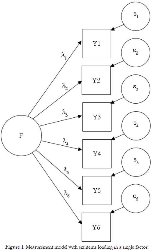
The construct is a latent variable, that is, not directly observable but inferred from the observable variables that are responses to items. The relationship between the construct and the item is linear and quantified by the factor loading (λ_j). Lambda is a measure of item discrimination interpreted as a regression coefficient: when there is an increase of one unit in the factor, there is an increase of λ_j units in the item j. Note that linearity is only appropriate for items that are normally distributed. Each item is also characterized by its difficulty index, quantified in CFA by the intercept or score in the item when the score in the factor is zero. Finally, the error term is unique for each item; it is uncorrelated with the factor score and also with the errors of the other items.

Setting the factor variance to 1 for model identification purposes, it can be shown (Jöreskog, 1971; McDonald, 1999) that the reliability of a score obtained as sum or mean of the items is:

or the ratio between the true score variance derived from estimated model parameters and the sum of item variances and covariances implied by the model. This estimator was labeled coefficient omega by McDonald, composite reliability by Raykov (1997), and internal consistency reliability estimated by SEM by other authors (e.g., Yang & Green, 2011) as CFA is part of SEM procedures. A more general equation based on a non-standardized latent variable can be found in Raykov (2012).

According to McDonald (1999), if the measurement model fits the data, Equation 2 can be rewritten substituting the denominator by the sum of observed item variances (σ_j²) and covariances(σ_j<ji):

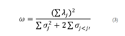
In fact, McDonald considers it even more convenient to use Equation 3. Other experts such as Bentler (2009) prefer Equation 2 as the covariance matrix reproduced by a model is a more efficient estimate of the covariance matrix population than the product-moment estimate. If the model fits the data, the practical consequences will be negligible. In contrast, if the model does not fit the data, we share McDonald's recommendation that none of the coefficient omega expressions should be used to estimate internal consistency reliability.

As seen below, omega is currently a family of internal consistency reliability coefficients derived from CFA parameter estimates. Most of these coefficients have been derived relaxing uncorrelated errors, normality and unidimensionality assumptions to accommodate real data properties. Alpha itself is a member of the family and based on very restrictive assumptions.

Reliability of essentially tau-equivalent measures

The omnipresent α is an unbiased estimator of internal consistency reliability provided that the essentially tau-equivalent measurement model fits the data (e.g., Jöreskog, 1971, McDonald, 1999). This model is depicted on the left of Figure 2. Note that the factor loadings of all the items have been equated. This reflects the assumption that all discrimination parameters are equal, that is, when controlling for the factor score difference between two groups of examinees, the difference of item scores between the two groups will be constant across all items.

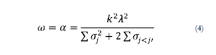
If essential tau-equivalence holds, the value of the coefficient omega is equal to the value of α which, in turn, equals other coefficients developed earlier for the same purposes such as the Guttmann's Lambda 3 (e.g., Revelle & Zinbarg, 2009). The numerator of previous Equation 3 in this case reduces to the product of the number of items squared (K²) by the factor loading squared (λ²). The unweighted least squares (ULS) estimator of the squared factor loading is the average covariance between the items and the denominator is the sum of observed variances and covariances between the items.

Consequently, if the essentially tau-equivalent measurement model fitted the data, it would be good practice to calculate a to provide an estimate of the internal consistency reliability of the sum or average of the items.

Reliability of congeneric measures

As anyone with experience in CFA knows, factor loadings of items are not usually equal at first sight. This fact is better modelized by the congeneric measurement model which permits different discriminative power across items. In fact, this is the general unidimensional factor model depicted in Figure 1 explained before. If the congeneric measurement model fits the data and the more restrictive essentially tau-equivalent model does not, the internal consistency of the sum or average of the items should be estimated using the coefficient omega in Equation 2 or in Equation 3.

The relationship between α and omega for congeneric not essentially tau-equivalent measures has been thoroughly studied. First of all, it has been shown that α is lower than omega and can thus be trusted as the lower limit of reliability (Raykov, 1997). Second, simulation studies have shown that the difference between a and omega has no practical consequences when factor loadings are on average .70 and the differences between them are within the interval -.20 and +.20 (Raykov & Marcoulides, 2015). Therefore, if these conditions are met, we can continue using α as the point estimator of internal consistency reliability, which may even be desirable for practical reasons, according to these authors. Otherwise, omega should be used as α would underestimate the internal consistency reliability, at least in the event of a statistically significant difference between α and omega (Deng & Chan, 2016).

Finally, simulation studies (Gu, Little, & Kingston, 2013), showed that neither the number of non-tau-equivalent items in a questionnaire nor the magnitude of the differences between factor loadings produce sizeable biases when using α to estimate population reliability. Larger biases are due to correlated errors and small ratios of true to error variance.

Reliability of measures with correlated errors

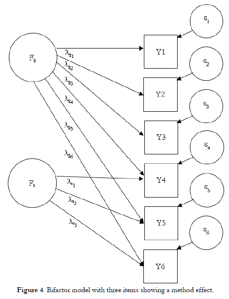
We turn now to measures where the uncorrelated errors assumption is not tenable. A well-known case occurs when a questionnaire contains items positively and negatively worded that measure the same construct. In this case, once the effect of the latent variable is controlled, the positively worded items still retain a not negligible covariance with each other, as do negatively worded items. This situation can be modelized specifying some correlations between errors other than zero (Figure 2, right; see e.g., Brown, 2015; Marsh, 1996) or as a method factor due to the composition of the questionnaire (Figure 4, see below and also Gu et al., 2013) or even as a parameter due to respondents' individual differences (Maydeu-Olivares & Coffman, 2006). For the sake of simplicity, in this section we will focus on the first and briefly refer to the remainder below when dealing with the assumption of unidimensionality.

 

 

If not taken into account, the presence of correlated errors has serious effects on internal consistency reliability estimation. Estimates of factor loadings are incorrect (e.g., Brown, 2015) and both omega and α are biased estimators of population reliability although the bias is much greater if a is used (Gu et al., 2013). In addition, α can no longer be trusted as the lower limit of reliability of scale scores (Raykov, 2001). In fact, depending on the parameter configuration of the measurement model, α bias could lead to underestimating or even worse, to overestimating population reliability, giving a false sense that scale scores are reliable when actually the opposite is true.

Bias should be corrected by including the covariance between errors in both the model parameter estimation and the omega formula, as shown below (Raykov, 2004; see Bollen, 1980 for the original unstandardized factor formulation):

The sum of the elements of the implied variance-covariance matrix in the denominator clearly illustrates the difference between Equation 5 and Equation 2. Again, if the model with correlated errors fits the data and thus model parameters have been correctly estimated, Equation 3 using the observed variance-covariance matrix in the denominator would provide very similar results.

The simulation studies by Gu et al. (2013) showed that, in the presence of correlated errors, alpha may overestimate population reliability with differentials as high as .38. This would mean, for instance, that a score with a true reliability of .40, which is completely unacceptable, may result in an a value of up to .78, which may lead to the erroneous conclusion of fairly good reliability. All conditions being equal, the omega coefficient corrected for correlation between errors gives a bias of -.09, practically negligible and therefore preferable. These authors conclude that α seems to treat the correlation between errors as if it were part of the true variance thus producing overestimation of reliability. We will return to this point below when dealing with the unidimensionality assumption.

Why and how to conduct the analysis

Incorrectly estimating reliability has undesirable consequences in all applied fields where questionnaires are used. In instrument development, reliability underestimation can lead researchers to make unnecessary improvement efforts, whereas overestimation brings unwarranted confidence to the questionnaire. Even if obtaining the lower limit of reliability could suffice for questionnaire development, it would not be enough for subsequent use. In basic or applied research, the effect sizes can be seriously affected if a biased reliability estimate is used to calculate the correction for attenuation (Revelle & Zinbarg, 2009). In individual decision making, a biased reliability estimate would affect the standard error of measurement, which can lead to inadequate decisions in interpretation and communication of scores.

When based in an internal consistency design, reliability estimation should be derived from a measurement model fitted using SEM methods. In this section we present a procedure in three analytic phases and postpone the discussion of the costs of such an analytical strategy until the final section of the paper.

Phase 1: Screening of the item responses. The univariate distributions and relations between items are studied in order to make decisions on variable types and possible item clustering that can affect model specification and estimation in the next phase.

Phase 2: Fitting the measurement model to the data. This is a confirmatory activity, therefore it starts by specifying the suitable models derived from prior knowledge of the questionnaire, continues estimating parameters and evaluating the goodness of fit and the adequacy of the solution for all suitable models. As a result, the measurement model with conceptual meaning and good fit to the data is chosen. For purportedly unidimensional questionnaires, the analyst should consider essentially tau-equivalent, congeneric and, perhaps, correlated error measurement models. These are nested models, the essentially tau-equivalent being the most restrictive model (i.e., with fewer free parameters to be estimated) and the correlated error model the least restrictive.

Phase 3: Calculation of the internal consistency reliability coefficient derived from the measurement model parameters and its standard error in order to provide an interval estimate of reliability.

Our proposal is aligned with those of other authors that suggest always performing Phase 2 and deriving from it the reliability estimation in Phase 3 of the analysis (e.g., Crutzen & Peters, 2015; Graham, 2006; Green & Yang, 2015). For the sake of correction, in addition to the two consensual phases we believe it essential to stress the implicit third stage in the analysis. A previous screening of the data should be carried out to correctly decide on the association matrix to be analyzed and the estimator of the measurement model parameters. See for example, the book chapters by Behrens, DiCerbo, Yel, and Levy (2012), Malone and Lubansky (2012) and Raykov (2012), or the papers by Lloret-Segura et al. (2014) and by Ferrando and Lorenzo-Seva (2014) in a previous issue of this journal. Put simply, in Phase 1 of the analysis the distributions of item responses and the relations among them should be analyzed to determine the type of data and to detect items differentially related to the others or item clustering. This phase will allow the analyst to decide whether to treat their data as quantitative or as ordinal/categorical, two options that will be addressed in the following two sections, and also to decide on a possible correction for correlated errors, whose treatment will be seen in more detail in the next section on practical scenarios.

Additionally, in Phase 3 we suggest giving an interval estimation of the reliability. Although it has been customary to publish the point estimate of internal consistency coefficients, it should be taken into account that they are statistical indicators obtained in a sample and thus affected by standard error. Consequently, the 95% CI should be published as usual in the social and health sciences. The standard error for reliability coefficients can be estimated by bootstrap (Kelley & Pornprasertmanit, 2016; Raykov & Marcoulides, 2016a) or approached using the analytical delta method (Raykov, 2012; Padilla & Divers, 2016). The less computationally demanding delta method provides results comparable to the bootstrap with nonbinary items and large samples (greater than 250 cases, Padilla & Divers, 2016).

Quantitative data analysis

Item responses obtained on a quantitative scale (e.g., visual analogue scale) are continuous, quantitative data. Responses obtained on a rating scale such as a Likert type scale, are ordered categories which can be analyzed as continuous variables provided that the number of categories is high (5 or more) and the frequency distribution does not show floor or ceiling effects (Rhemtulla, Brosseau-Liard, & Savalei, 2012). This is the main decision to be taken in Phase 1.

All plausible measurement models for the data at hand would be specified using CFA in Phase 2. At the very least, essentially tau-equivalent and congeneric measures should be considered. Next, the model parameters will be estimated, goodness of fit indices calculated, and the best fitting, parsimonious and interpretable measurement model will be chosen. The estimated parameters will be used to obtain the internal consistency reliability in the next phase. All these operations can currently be performed quite easily using commercial software such as Mplus (Muthén & Muthén, 2017) and also the free software environment R (R Core Team, 2016). See next sections for examples and syntax in R.

We outline here the procedures for model fitting in SEM but the full details exceed the objectives of this paper. See references such as Abad, Olea, Ponsoda and García (2011), Brown (2015) or Hoyle (2012) for an indepth treatment on parameter estimation, model fit, model comparison and revision.

Either the full data matrix of cases by items or the covariance matrix between items will be analyzed. If the multivariate normal distribution holds, the maximum likelihood estimation method (ML) will be used and the goodness of fit tested using global and local fit indicators. A statistically null value of χ² together with parameter values and standard errors within acceptable range would provide evidence favoring the measurement model being tested. Complementarily, decision-making can be supported using approximate fit indices, such as the comparative fit index (CFI), the TuckerLewis index (TLI) and the mean square error of approximation (RMSEA), all ranging between 0 and 1. Roughly speaking, the values of CFI and TLI should be greater than .95 and that of RMSEA less than .05 for the model to be considered appropriate.

Nested models can be compared based on χ² difference between them. This formal comparison can also be complemented evaluating the differences between the approximate fit indices. It is generally considered that two nested models fit equally well to the data if the difference in χ² is statistically non-significant and also if the differences between the approximate fit indices are less than .01.

Minor deviations from normality, even in the case of ordered categories not presenting floor or ceiling effects, can be handled using the robust maximum likelihood estimation (MLR) and associated χ², CFI, TLI and RMSEA indices. Parameters are still estimated using normal theory ML, but standard errors and overall fit indices are corrected for nonnormality. However, the comparison between nested models is not so direct, since the difference between corrected χ² values is not interpretable. Satorra-Bentler or Yuan-Bentler correction factors should be applied (Muthén & Muthén, n.d.).

Regardless of the estimator used, Phase 2 of the analysis concludes choosing the most parsimonious model with conceptual sense and good fit to data. During Phase 3 of the analysis the estimated parameters will be used to calculate the alpha or omega coefficients when appropriate and the standard error will be obtained using bootstrap in general or delta method in large samples in order to provide an interval estimate.

Ordinal and dichotomous data analysis

Many questionnaires have categorical response formats, with two (e.g., Yes / No) or more options (e.g., Strongly Disagree / Disagree / Agree / Strongly Agree). Therefore, the analyst often faces binary or graded/ordered categorical data. In Phase 1 of the analysis, special attention will be paid to the number of response categories that have actually been used by respondents and also to the distribution form. If the number of response categories is four or less, or even with five or more response categories showing prominent ceiling or floor effects, the parameter estimation in the next phase can no longer be approximated by normal theory based estimators. An appropriate estimator for categorical data should be used instead, again according to the recommendation by Rhemtulla, Brosseau-Liard and Savalei (2012) also mentioned in the previous section.

To conduct Phase 2 of the analysis, the analyst can choose between three options (e.g., Bovaird & Koziol, 2012). The first is to aggregate multiple items before analysis (parceling), which provide quantitative data to be analyzed. This solution remains very controversial (Little, Rhemtulla, Gibson, & Schoemann, 2013; Marsh, Lüdtke, Nagengast, Morin, & Von Davier, 2013) and is only credible if stable between different, equally plausible forms of parceling items (Raykov, 2012). The second option is keeping the analysis at the item level and estimating the parameters of a plausible item response theory (IRT) model for these data. This strategy uses full information estimation (based on response patterns) and can be applied to one, two, three or four parameter models. The third option is still item-level analysis but the limited information estimation (based on polychoric or tetrachoric correlation matrix) of CFA is used for one and two parameter models. We adopt the third option in this paper as it facilitates the generalization of the concepts dealt with up to now and is equivalent to some of the most usual normalogive IRT models (e.g., Cheng, Yuan y Liu, 2012; Ferrando & Lorenzo-Seva, 2017).

The model for categorical item responses is depicted in Figure 3. To account for ordinality, a latent continuous response distribution (Y_j) is defined that leads to an observed ordered categories distribution (Y_j). The latent response is related to the observed response through discrete thresholds (Muthén, 1984). In other words, when there is a change in Y_j* that crosses the threshold between two response categories, the discrete observed value of the observed variable Y_j changes to the adjacent category. The cumulative normal distribution is usually taken as a link function between thresholds and cumulative proportions of responses. Otherwise, the latent model for Y_j* is the same as the model in Figure 1. Therefore, the measurement models to be considered will still be those of essentially tau-equivalent measures, of congeneric measures and the model of measures with correlated errors. Changes occur only in estimation techniques. Nowadays, most statistical packages for SEM include options to correctly fit measurement models for ordinal data. Again, the commercial software Mplus and the free software environment R are among the most popular. See sections below for a developed example and syntax in R.

 

 

As with quantitative data, an outline of the procedure for Phase 2 follows. See references such as Brown (2015), Hancock and Mueller (2013), or Hoyle (2012) for a more indepth treatment. The procedure begins with the estimation of the polychoric correlation matrix for items with three or more categories, or tetrachoric correlation for dichothomus items. Secondly, the measurement model is fitted to this correlation matrix using an estimation method appropriate to the categorical nature of the variables. The most suitable estimation method for a wide range of sample sizes is robust weighted least squares with a mean and variance adjusted χ² statistic (WLSMV, e.g., Bovaird & Koziol, 2012), even if for small samples (close to 200 cases) the ULS method can be a good alternative (Forero, Maydeu-Olivares, & Gallardo-Pujol, 2009). The interpretation of results including the goodness of fit indices and the comparison of nested models still require more training in this case, so we strongly recommend consulting the mentioned specialized texts and being up to date regarding new developments in this field (e.g., Huggins-Manley & Han, 2017; Maydeu-Olivares, Fairchild, & Hall, 2017; Sass, Schmitt, & Marsh, 2014).

Once the estimates of the model parameters are obtained, the internal consistency of the sum of latent item variables Y_j* can be estimated from the ordinal omega coefficient (Elosua & Zumbo, 2008; Gadermann, Guhn, & Zumbo, 2012). Consistent with Equation 2, these authors propose calculating the coefficient from the estimated parameters, both in the numerator where the true score variance would be obtained from the estimated factor loadings, and in the denominator where the true plus error variance would be obtained by the sum of the elements of the implied polychoric correlation matrix. As is customary, if the model fits the data well, the elements of the polychoric correlation matrix in coherence with Equation 3 can be used. Additionally, being the sum of elements of a correlation matrix the denominator can be simplified, so for a questionnaire with k congeneric measures ordinal omega reduces to Equation 6 where P*_j<ji refers to the polychoric correlation coefficients:For essentially tau-equivalent measures the ordinal alpha coefficient can be used (Elosua & Zumbo, 2008; Gadermann et al., 2012; Zumbo, Gadermann, & Zeisser, 2007), where the numerator is simplified in coherence with Equation 4: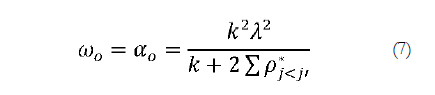As occurs with α for quantitative data, the ordinal alpha coefficient is only recommended if an essentially tau-equivalent model underlies the data, while the ordinal omega coefficient is recommended if the underlying model is that of congeneric measures (Gadermann et al., 2012; Napolitano, Callina, & Mueller, 2013). Once again, the bias using ordinal alpha would be more serious when correlated errors had not been specifically addressed in the model, as they would be included in the numerator as part of the true variance.

Ordinal coefficients are advantageous in that they constitute a straightforward generalization of linear omega coefficients, but are limited as they do not assess the reliability of the observed item sum or mean (Y_j), but that of the underlying latent continuous responses (Y_j*). If the researchers are interested in the reliability of the item sum, a better choice is the nonlinear SEM reliability (Green & Yang, 2009; Yang & Green, 2015). The conceptual formula is close to that of ordinal omega, but the normal cumulative probability of the thresholds is included both in the numerator and in the denominator in order to express the true and error variances in the metric of the observed item sum. The actual calculation is complex, therefore the authors provide the SAS code in an appendix (Green & Yang, 2009). CI for nonlinear SEM reliability coefficient can also be obtained using R (Kelley & Pornprasertmanit, 2016) provided that the congeneric measurement model is acceptable.

In the event that researchers chose to fit an IRT measurement model, the internal consistency reliability could still be derived from the estimated parameters. As in the case of CFA, the IRT models provide estimates of the item parameters and the distribution of the latent variable that allow quantifying variance of the total scores, true scores and errors as conceived in the CTT (Kim & Feldt, 2010 and references therein), and from these variances reliability can be estimated as the ratio of true score variance over total score variance as defined in Equation 1.

For unidimensional dichotomous data and a congeneric measurement model, Dimitrov (2003) developed the point estimation of the internal consistency reliability for one, two or three parameter models, provided that the items had been previously calibrated. To avoid computational complexities, Dimitrov proposed using approximate calculations so that the formulas can be easily implemented into a spreadsheet, basic statistical programs or programmed in R. Raykov, Dimitrov and Asparouhov (2010) further developed these ideas by incorporating them into a method that simultaneously allows the item calibration and the interval estimation of internal consistency reliability for the item sum both for one and two parameter models. As customary, they provide the syntax for Mplus users to estimate the model parameters and the CI of internal consistency reliability in a single run.

Application to four practical scenarios

To illustrate the above concepts, we present four examples which mimic applied research situations where the sum or mean of responses to multiple items are aimed at measuring a single construct. In each of the four scenarios, we analyzed the simulated responses of 600 people to 6 items in a five-point Likert scale. A noticeable difference with applied research is related to the origin of prior knowledge regarding compatible measurement models. In applied research this necessary prior knowledge proceeds from the underlying theory and previous studies, whereas in our examples it comes from the knowledge of the underlying simulated models.

In Case 1 an essentially tau-equivalent measurement model with high factor loadings close to .65 underlay the data, and the response distributions were symmetric. Accordingly, it was expected that descriptive statistics would suggest analyzing data as quantitative, that the essentially tau-equivalent measurement model would be the best fitting model, and that the omega value would be equal to alpha value. In Case 2, the underlying model was the congeneric measurement model with homogeneously high factor loadings and symmetric response distributions. Consequently, it was expected that item responses could be treated as quantitative, the best fitting model would be congeneric measurement model, and alpha would be expected to be close to omega due to the homogeneously high factor loadings. In Case 3, the underlying model had highly variable factor loadings plus three items with correlated errors, response distributions still being symmetric. Therefore, there were three expectations, descriptive statistics to support a quantitative subsequent analysis, the best fitting model to be that of measures with correlated errors, and alpha value to be unduly greater than omega mainly due to the fact that omega corrects for the correlation between errors whereas alpha treats this correlation as true variance. Finally, in Case 4 the underlying model was congeneric measurement model with highly variable factor loadings and with strong ceiling effects in the response distributions. In this case, it was expected that descriptive statistics would suggest treating data as ordinal and that the congeneric measurement model would show the best fit. Regarding the two reliability coefficients, they are expected to show a sizeable difference as ordinal alpha estimates the reliability of essentially tau-equivalent latent responses, whereas the non-linear SEM reliability coefficient estimates the reliability of congeneric observed responses.

The analyses were carried out using R. Phase 1, descriptive analysis, was conducted using the reshape2 (Wickham, 2007) and psych (Revelle, 2016) packages to calculate the response percentages, other descriptive statistics, and the Pearson or polychoric correlation coefficients when appropriate. In Phase 2, the nested measurement models were analyzed using the cfa function from the lavaan package (Rosseel, 2012) choosing the ML estimate in the first three cases, as per quantitative data, and the WLSMV estimate in Case 4, as per ordinal data. In order to facilitate comparison, in Phase 3 both a and omega coefficients were obtained for the best fitting parsimonious measurement models using the reliability function of the semTools package (semTools Contributors, 2016). When available, the 95% confidence intervals were calculated using the ci.reliability function of the MBESS package (Kelley & Pornprasertmanit, 2016). All decision making was based on the criteria described in the previous sections. The data for the examples are available at http://ddd.uab.cat/record/173917 and the syntax used can be found in Appendix A and Appendix B of this paper.

Table 1 presents univariate and bivariate descriptive statistics for all scenarios. In Case 1, the central categories showed the highest percentage of responses and no ceiling or floor effects were observed. The values of skewness ranged between -0.11 and 0.10, and those of kurtosis between -0.29 and -0.64, so that the data were treated as quantitative although they proceed from the responses to a five-point Likert scale. All Pearson correlation coefficients were positive and homogeneous ranging from .31 to .47. Therefore, we decided to test the two plausible measurement models, congeneric versus essentially tau-equivalent, using the ML estimator. The results are presented in the first two lines in Table 2. The most constrained model tested, the essentially tau-equivalent measurement model, showed good fit to the data, χ² (14) = 22.02, p = .078, CFI = .992, TLI = .991, RMSEA = .031. As the χ² difference with the more flexible congeneric measurement model was not statistically significant, χ² (5) = .09, p = .999, we chose the essentially tau-equivalent measurement model in application of the parsimony principle. Thus, all assumptions were met for α (see Equation 4) to be a good estimator of internal consistency reliability. As expected, the α estimate of .809 was the same as the omega estimate. The internal consistency of the sum or average of the items in Case 1 was within the usual standards with 95%CI values between .784 and .831.

The exploration of the data in Case 2 also led us to treat them as quantitative. Indeed, descriptive statistics in Table 1 showed the frequencies on a five-point scale without ceiling or floor effects, with skewness not higher than 0.19 in absolute value, kurtosis not higher than 0.85 in absolute value, and homogeneous correlation coefficients between items in a range between .26 and .53. In consequence, the congeneric and essentially tau-equivalent measurement models were tested using the ML estimator. As seen in Table 2, unacceptable fit was obtained when the constraint of equal factor loadings was imposed (essentially tau-equivalent measures), χ²(14) = 46.78, p < .001, CFI = .969, TLI = .967, RMSEA = .062. A considerable improvement in fit was observed when factor loadings were allowed to be different across items in the more flexible congeneric measurement model, χ² (9) = 20.46, p = .015, CFI = .989, TLI = .982, RMSEA = .046. Moreover, the χ² difference between both models was statistically significant, χ² (5) = 26.32, p <.001, indicating a better fit of the congeneric measurement model. Thus, in this case, internal consistency estimates should be obtained using the coefficient omega (see Equation 2). However, as already anticipated, both the coefficient omega (.823) and the coefficient alpha (.820) showed similar values as all factor loadings were homogeneously high (between .60 and .83). The minimum values of both CIs were well above the usual standards, constituting evidence in favor of the internal consistency of the scale scores.

Again, in Case 3 all descriptive statistics suggested analyzing data as quantitative. The response distributions in five categories did not show extreme responses and the skewness and kurtosis indices were not higher than the absolute values of 0.17 and 0.51 respectively (see Table 1) and therefore the ML estimator was deemed appropriate. However, as expected, the correlation coefficients were not homogeneous since very high correlations, greater than .78, between three items (Y4, Y5, Y6) were observed, while the remaining correlations ranged between low and moderate from .05 to .43. These three items showed a special clustering that would be modeled as correlated errors.

As shown in Table 2, the fit of the essentially tau-equivalent measurement model was not acceptable, χ² (14) = 608.25, p < .001, CFI = .669, TLI = .645, RMSEA = .266. The goodness of fit indices for congeneric measurement model, although better, χ² (9) = 78.19, p < .001, CFI = .961, TLI = .936, RMSEA = .113, were not acceptable, with the exception of the CFI. Modeling the high correlations between items Y4, Y5 and Y6 as correlations between their errors, good fit indices were observed, χ² (6) = 13.82, p = .032, CFI = .996, TLI = .989, RMSEA = .047, except for the statistically significant χ². Additionally, a statistically significant difference with congeneric measurement model was found, χ² (3) = 64.37, p < .001, indicating that the model with correlated errors presents a significantly better fit than the congeneric measurement model.

In coherence with the fitted measurement model, the internal consistency estimate was obtained with the coefficient omega corrected for correlated errors (see Equation 5). The observed value of .560, well under the usual standards, leads to the conclusion that the item sum is not a reliable measure. This conclusion is consistent with the result of Phase 2, where unidimensionality was seriously put into question. Both results show that the raw sum scores are not an appropriate measure in Case 3. The fact that the essentially tau-equivalent measurement model did not fit the data, and especially the presence of items with correlated errors, should discourage the use of α to estimate internal consistency reliability. Nevertheless, α was included in Table 2 to illustrate the dramatic changes in the conclusion in case α was used, as its value of .773 would have easily led to the incorrect belief that the items were consistent.

The distribution of responses in Case 4 showed very clear ceiling effects with all items showing more than 60% of cases piled in the last response category, as seen in Table 1. Although skewness and kurtosis values did not particularly stand out, they were out of the range between -1 and 1. Consequently, even if the data came from a five category response scale, the response distribution suggests the convenience of considering them as ordinal. For this reason, poly-choric correlation coefficients were calculated, with quite a large range of values between .19 and .64 being observed, but no particular clustering of items. For the same reason, the WLSMV estimator was used to test the fit of the congeneric and essentially tau-equivalent measurement models to the data.

As observed in Table 2, the fit to the essentially tau-equivalent measurement model was unacceptable, χ² (14) = 100.78, p <.001, CFI = .950, TLI = .946, RMSEA = .102, while it was good for the congeneric model, χ² (9) = 20.07, p = .018, CFI = .994, TLI = .989, RMSEA=.045, except for the statistically significant χ² value. Thus, we chose the congeneric measurement model as the most suitable for these data. In coherence with the fitted measurement model, the proper estimator was the nonlinear SEM reliability coefficient (see Green & Yang, 2009) with a value of .777, 95% CI [.739, .808]. These values are within accepted standards in the scale development process. With the ordinal alpha coefficient (see Equation 7) a clearly superior value of .830 would have been obtained although it would be incorrect as the tau-equivalence condition is not met. Moreover, ordinal alpha estimate the reliability of the sum of latent response variables and not the reliability of the sum of observed responses.

Generalization to complex measurement models and designs

In this section the previous rationale and results are generalized to essentially unidimensional measures, to multidimensional scales, to multilevel designs and to data with missing values, as well as to the use of reliability coefficients in scale development and revision.

Reliability of essentially unidimensional measures

All models discussed so far share the assumption that the items measure a single construct. The presence of correlation between items after controlling for the common factor, as in Case 3, is treated as an anomaly to be corrected. However, this is a particular case of a more general topic. Each item can measure both the intended construct and other factors that the researchers consider spurious. Possible reasons include questionnaire characteristics, such as the positive or negative wording of the items or the presence of testlets, and also response biases such as social desirability, negative affect or acquiescence (e.g., Conway & Lance, 2010; Lance, Dawson, Birkelbach, & Hoffman, 2010; Spector, 2006). In this section we will use the concept of essential undimensionality coined by Stout (1987; see also Raykov & Pohl, 2013) to discuss a more general way of treating questionnaires that predominantly measure one factor but where additional spurious factors formed by item subgroups can be identified.

When spurious sources of variability are suspected, the analyst can detect some item clustering through careful observation of the correlation matrix during Phase 1 of the analysis, as illustrated in Case 3. However, the formal analysis is conducted in Phase 2. The specification of a bifactor type measurement model (e.g., Reise, 2012) is particularly useful for determining essential unidimensionality. In this model, depicted in Figure 4, each item is allowed to load on a general factor and also on a group factor that might be spurious. More than one group factor can be defined to accommodate various item clusters. If the bifactor model fits the data and the researchers believe the group factors to be spurious, then they should include this knowledge in Phase 3 of reliability estimation. The appropriate coefficient labelled hierarchical omega by Zinbarg et al. (2005) and applied to the diagram of Figure 4 is: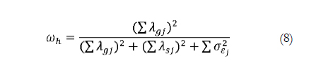The true variance in the numerator is derived from the general factor, whereas the variance due to specific factors is treated as error variance by being included only in the denominator. This formulation excludes all spurious variance from the numerator of the reliability coefficient, whether attributable to method factors, item specificities, response process or random variation. Provided that the model fits the data, the sum of observed variances and covariances can be used in the denominator, as discussed on presenting Equation 3. Omega hierarchical is a more general specification for Equation 5 as is explained by Gu et al. (2013) for quantitative data and by Yang and Green (2011) for ordinal data.

If previous knowledge regarding possible sources of spurious variance is available, a confirmatory bifactor model can be specified and fitted using the lavaan package in R or the commercial software Mplus. If researchers wish to provide evidence of unidimensionality in the absence of previous knowledge regarding particular sources of spurious variance, an exploratory bifactor model can be conducted using Schmid-Leiman or Jennrich-Bentler rotations (e.g., Mansolf & Reise, 2016) using the psych package in R or the commercial software Mplus. This general exploratory approximation is more adequate than the somewhat usual practice of parameter respecification based on local modification indexes derived from a misfitting congeneric measurement model (see e.g., Brown, 2102; Hoyle, 2102).

As reasonable as it sounds, this is only one of the two conceptualizations of internal consistency reliability based on SEM (Zinbarg et al., 2005). These are derived from the fact that conceptually, in factor analysis, the observed score can be attributed to four sources of variability, namely, a general factor in which all items would load on, group factors formed by subgroups of items, factors specific to each item, and random variation. In contrast, in CTT, the observed score is only divided into two parts: true and error scores. Consensus exists in that the general factor is part of the true variance and random variation is part of the error variance. Group factors due to different item contents would also be considered true variance and would make the questionnaire multidimensional. The different conceptualizations of reliability come from whether the spurious group factors and the specific factors can be considered part of the true variance or the error variance. The answer given on calculating hierarchical omega is that spurious and specific variability, which are not part of the construct, are part of the error variance.

On the other hand, a more classic conceptualization of reliability would sustain that all systematic factors contribute to the correlations between items and, even more importantly, to correlations with external variables; only random errors have the effect of attenuating these correlations. Therefore, the reliability of the item sum or mean scores should include all systematic variation, whether due to either content, method or specific factors. This is all the more so if we wish to still consider the reliability coefficient as the upper limit of the predictive validity coefficient. Researchers who identify with this position will favor calculating internal consistency reliability through the coefficient that Zinbarg et al. (2005) called omega total and whose expression applied to the example of Figure 4 is: 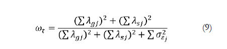In omega total the group factor is considered part of the true variance and is therefore included in the numerator. As Bentler (2009) warned, the decision to consider spurious and specific factors as part of the true or error variance depended on the researchers' objectives. In a single administration of a questionnaire intended to measure one construct, the discussion is circumscribed to the possible spurious group factors, as the factors specific to each item cannot be distinguished from the random variation.

In this context, the proposal of Green and Yang (2015) to publish both omega hierarchical and omega total seems reasonable. This allows not only evaluating the reliability under the two conceptualizations, but also gives a simple assessment of the unidimensionality. A high similarity between the two values would yield favorable evidence for unidimensionality, as the spurious factors would not provide much systematic variance. Both omega hierarchical and omega total can be obtained based on confirmatory bifactor modeling using Mplus or the lavaan and semTools packages in R. Their exploratory versions can be obtained using the omega function of the psych package of R.

Additionally, in longitudinal designs the item specific factors can be identified and a range of solutions has been proposed to take them into account. McCrae (2014) maintained the position that it would be more appropriate to attend to test-retest reliability since it certainly includes item specificity, whereas Bentler (2016) proposed specificity-enhanced internal consistency indices and Raykov and Marcoulides (2016b) provided the rationale and syntax for the estimation of specific variance in SEM analysis using the Mplus software.

Finally, we would like to highlight that equations from Equation 2 to Equation 10 are pertinent to estimate reliability when planning to use the sum or mean of items for later predictive, group comparison or longitudinal analyses. These are linear combinations with equal weights for all items. However, if the aim is to study relationships between latent variables in an SEM model, the constructs would be measured through the optimal linear combination of their indicators, so that their internal consistency reliability would be more adequately estimated by the coefficient H (Hancock & Mueller, 2001, 2013) also known as maximal reliability (Raykov, 2012). The ratio between the communality (λ²_j) and specificity (1 - λ²_j) of each item is the core of coefficient H. The coefficient can be interpreted as the maximum proportion of variance of the theoretical construct that can be explained by its indicators, or put differently, the reliability of the optimal linear combination of items. Among its properties, we highlight that H is equal to or greater than the reliability of the most reliable item, it does not depend on the sign of the factor loadings nor does it decrease when the number of items increases. Equation 10 is only adequate if the essentially tau-equivalent or the congeneric measurement model fit the data. If a measurement model with correlated errors is used, the coefficient should be corrected accordingly (Gabler & Raykov, 2017). On the other hand, if an IRT based latent score was calculated, reliability should be obtained accordingly (e.g., Cheng, Yang y Liu, 2012).

However, estimating structural effects between latent variables using SEM methodology comes with its own drawbacks as the use of optimal linear combination provides measures that are dependent on the sample and the particular time point (e.g., Raykov et al., 2016). These authors suggest using this more complex measure only if absolutely necessary, that is, when the reliability of optimal linear combination (coefficient H, Equation 10) is statistically greater than the reliability of unit weighted linear combination (coefficient omega, Equation 2).

Reliability in multidimensional measures

So far, we have focused on unidimensional measurement scales perhaps affected by spurious factors, leaving out a wide range of useful measurement models. For example, how to calculate the internal consistency reliability of scores derived from multiple perhaps correlated factors? This is the case for numerous scales in the social sciences. An example of this would be a motivation measure, which will include at least one scale of intrinsic motivation, another of motivation oriented externally and perhaps a third of lack of motivation. For theoretical reasons, these constructs are expected to be correlated with each other, some positively and others negatively. But also, how to calculate the internal consistency reliability of scores derived from a hierarchical measurement model, with a general factor and some group factors with interpretable content? Classic examples are measures of a general intelligence factor plus specific factors such as verbal intelligence, logic, manipulative, etc. Or even more difficult, what to do if the entire questionnaire is made up of complex items? We refer to items that systematically show low cross loadings in several factors besides a higher factor loading in the intended factor (Marsh et al., 2010), as for example, personality tests such as the Big Five Test.

When faced with these structures, the data analyst could still find it useful to follow the procedure in the three previously described analytic phases. Probably, during Phase 1, exploratory, some clusters of variables can be observed, but the formal test for multidimensionality will be carried out in Phase 2, when studying the fit of the measurement model. Empirical evidence can favor a model with multiple orthogonal factors or with multiple correlated factors, a bifactor model, or even a second order factor model (e.g., Ntoumanis, Mouratidis, Ng, & Viladrich, 2015). As in unidimensional cases, it is essential that the adopted measurement model has theoretical sense and fits the data. Rules to conduct Phase 3, the calculation of the coefficient omega applied to the particular multidimensional scale of interest, will easily be found in or derived from the current literature. To give some examples, Black, Yang, Beitra, and McCaffrey (2015) explain how to calculate reliability in second-order and bifactor factorial models applied to an intelligence test; Gignac (2014) the reliability of a general factor coming from a multidimensional scale; Green and Yang (2015) the reliability of specific factors, applicable to the study of reliability of correlated factor models; Raykov and Marcoulides (2012) reliability and criterion related validity of multidimensional scales; Cho (2016) the coefficient omega in several multidimensional models for quantitative data; or Rodríguez, Reise, and Haviland (2016) how to calculate and interpret reliability coefficients derived from bifactor models.

Reliability in complex designs: missing data and multilevel designs

Another issue to be addressed is how to treat the data characteristics derived from the research design and the field study. In this regard, researchers may ask: How to calculate the internal consistency when individuals are nested in clustering structures such as classrooms, schools, teams or companies, providing multilevel data? And when the data are incomplete? Our answer would be that the analytical procedure in three phases still works under these conditions. That is, provided that the parameters of the measurement model are correctly estimated, a natural consequence will be that the reliability estimate based on these parameters would be correct.

In the case of multilevel data, in Phase 1 the intraclass correlation coefficient can be added to the analysis in order to assess the magnitude of the clustering effect. In Phase 2, the appropriate correction for clustering should be used, for example, adding the syntax line analysis: type = complex in Mplus. Once parameters are correctly estimated, in Phase 3, the reliability coefficient can be obtained using the equations presented in previous sections. An application to multilevel data can be found in the paper by Raykov, West, and Traynor (2015). These authors present all details to calculate alpha with MLR estimation and standard errors corrected by clustering including the syntax in Mplus. A generalization useful for the analysis of heterogeneous populations can be found in Raykov and Marcoulides (2014).

On the other hand, confronting incomplete data requires more nuanced strategies. In the first place, extreme caution should be exercised in the design of data collection and during field study, as the best way to deal with missing data is not to have it at all on reaching the analysis stage. Even so, specific methods are needed when analyzing a possibly incomplete database. The details surpass the objectives of this paper and can be found in the methodological literature (e.g., Enders, 2010, 2013; Graham, 2009), but an outline will be presented here. In Phase 1, the proportion of missing data should be assessed, as small amounts do not have serious consequences in subsequent analyses. If a moderate proportion is present, it is recommended to explore and discuss their structure, as data missing at random also have no major effects on SEM results if an ML parameter estimator is used. Finally the most elaborate strategies would be necessary in case the proportion is large and/or not at random. An example of missing data not at random can be found in the evaluation of the effectiveness of a treatment, in the case where some participants abandoned treatment due to it not having met their expectations. One of these strategies, the inclusion of auxiliary variables, is explained in the paper by Raykov and Marcoulides (2015) where, as usual, these authors include the Mplus syntax to calculate the reliability of the scale scores and their CI. Another option is the coefficientalpha package developed in R and documented in Zhang and Yuan (2016) that allows estimating the coefficients alpha and omega and the corresponding CI in the presence of missing data and of deviant cases in a manner consistent with the methodology of analysis presented here although only applied to a restricted range of measurement models.

Change in reliability due to scale revision

Scale development has been another popular use of the coefficient alpha. Although validity arguments are much more important when constructing a scale, once an item pool is relevant and representative to measure a construct, an effort can be made to select the subset with greater internal consistency. The contribution of an item to the reliability of the sum scores was traditionally assessed using the indicator known as "alpha if deleted", which consists of evaluating the change in reliability due to the item elimination. Again, an alpha-based indicator is not recommended as it would bring to scale development all the previously mentioned issues regarding reliability estimation. Fortunately, the coefficient omega can be used to calculate the internal consistency reliability of the scores obtained with any subset of items and, in particular, for all items except that whose contribution to the set we wish to study.

The specific procedure was developed by Raykov and his colleagues in three successive papers. The initial development for items with a quantitative response scale (Raykov, 2007), was later generalized for dichotomous data (Raykov et al., 2010) and finally, to more general conditions, namely, non-normal data, multidimensional scales, presence of correlated errors, or missing data (Raykov & Marcoulides, 2015). Following their custom, the authors include appendices containing the syntax needed in the Mplus commercial package. Presented below is a procedure distilled from the ideas of the three articles.

First, a reference value should be fixed for the desired reliability of the scale. This can be given by normative knowledge (e.g., an internal consistency greater than or equal to .70) or by previous studies in the field (e.g., to emulate the internal consistency of a scale published in another culture) or can be derived from data obtained using the scale in its current state of development. Next, the measurement model will be fitted and coefficient omega for total scores can be obtained if desired. The next step would be to use parameter estimates to calculate omega for the subset formed by all but the first item, and replicate the calculus for each and every item so an indicator "omega if deleted" would result for each item. These indicators could be compared visually with the chosen reference value analogously to the usual procedure used with "alpha if deleted". However, Raykov and his colleagues propose making decisions based on the CI of the difference between the reference coefficient minus the "omega if deleted" coefficient. The contribution of an item to the internal consistency is relevant if the CI of the difference does not include the zero value. Taking into account the mentioned order to calculate the difference, the interpretation would be as follows: in case the CI is completely below zero, the item is useful, since if eliminated, the scale loses reliability. In case the CI is entirely above zero, then it is preferable to exclude the item since its presence worsens the total reliability.

Concluding remarks: Returning home with new ideas for data gathering and analysis

The aim of this work has been to facilitate the incorporation of the most recent psychometric knowledge about the estimation of internal consistency reliability of measures obtained using questionnaires into the daily work of researchers and reviewers in the fields of social and health sciences. To do this, we have first examined the reasons for using α or the coefficient omega in estimating the internal consistency reliability in unidimensional scales. We have furnished two types of methodological reasons for decision making, some based on the measurement model underlying the data and others based on simulation studies on the bias of using either coefficient. Secondly, we have offered a practical guide to developing the analysis, providing the necessary syntax in the free software environment R and have commented on the results of several examples. Finally, we have outlined the main ideas for the application of the basic concepts to the analysis of dimensionally complex questionnaires, to multilevel designs with missing data, and to scale development. In this concluding section, we draw some practical consequences for the design, data collection procedures, and data analysis derived from the reasoning throughout the paper.

When preparing the popular one-test one-administration design for data collection, the researchers make decisions that will definitively condition future data analysis and results. We would like to highlight three of them, namely, the sample size determination, the gathering of predictive covariates of missing data, and devising of procedures to attend to response process and completeness of data.

The determination of the sample size for reliability estimation needs to be put into context. On the one hand, reliability of measures is usually estimated within a pilot study with relatively few cases and the naive use of alpha can give grossly biased estimates. On the other hand, the more correct estimates based on SEM methods require large samples in order to achieve stable results (Yang & Green, 2010) therefore the costs for the pilot study could rise disproportionately due to the adoption of this methodology. Thus, before thanking alpha for its services and using SEM derived estimators henceforth (McNeish, 2017) or completely avoiding SEM models due to their difficulties (Davenport et al., 2016) it is worth carefully considering when we need to shift from alpha to omega. The knowledge of the questionnaire and its psychometric performance in previous studies can greatly help to limit the cost of the pilot study without compromising the correct estimation of the reliability. According to the results of simulation studies discussed throughout this paper, α is quite a good reliability estimator for congeneric models with high factor loadings and a large number of items (Gu et al., 2013; Yang & Green, 2010). The main threat to a correct reliability estimation comes from unmodeled correlated errors or method effects, a threat which worsens with low factor loading to error ratios (Gu et al., 2013) and in measures based on a small number of items (Graham, 2006).

Consequently, in the event the previous psychometric data showed high factor loadings for all items in one factor without any spurious effects, it would be pertinent to opt for a first approximation to the internal consistency reliability estimation using α. A more comprehensive analysis of the measurement model could be postponed until obtaining data from the main study, which will normally be based on larger samples which are more suitable for this purpose. This strategy would keep the sample size and the costs of the pilot study within reasonable limits.

On the contrary, if the questionnaire contained a few items per measure, or if there were any doubts regarding the size of the factor loadings or the unidimensionality, it would be safer to estimate internal consistency reliability starting from the appropriate measurement model using SEM methodology and thus collecting larger samples from the beginning. Finally, in case previous results compromised the quality of the measure, it would be good to have in mind this information at the design stage when still deciding on the measures to be included in the main study and consider the opportunity to include further development of the measure in the pilot study.

Regarding missing data and response processes, although robust statistical methods have been developed to face both incomplete data and response biases, the best time to address them is during the data gathering stage. All efforts should be made to facilitate the respondents' participation in order to increase the quality of the data and ultimately of the conclusions. Additionally, it is advisable to record possible predictors of missingness. As we have seen (see also Raykov & Marcoulides, 2015), their inclusion in subsequent analyses will allow correcting the bias due to missing data not randomly distributed.

Turning to data analysis, in Figure 5 we present a decision diagram synthesizing the ideas developed in previous sections. Coherent with the approach taken in this paper, we propose conducting the analysis in three phases. During Phase 1, the analyst should consider the sample size, the response scale format, and the results from the exploration of the univariate distributions and of the relationships between the items. The first decision, based on the response distributions, would be whether the data should be treated as quantitative or ordinal/categorical. When the response scale is quantitative and responses are normally distributed, model parameters will be estimated from the variance-covariance matrix through an ML estimator. When the number of categories in the response scale is equal or above five and no clear ceiling or floor effects are observed, the data can be treated as quantitative. Variance-covariance matrix will be analyzed generally using an ML estimator. Minor deviations from normality can be managed correctly using a robust estimator for the standard errors (MLR). In contrast, data should be treated as ordinal/categorical if the response scale has less than five categories or even five or more categories and the response distributions present piling of cases at the scale end. Polychoric or tetrachoric correlation matrix will be analyzed generally using the WLSMV estimator, or the ULS estimator with small sample sizes.

Phase 2 of the analysis consists of fitting the measurement model. The decision is whether to choose the best fitting parsimonious measurement model with theoretical sense. In line with this paper, in Figure 5 the analysis begins with the more restrictive model, the essentially tau equivalent measures model, and progresses relaxing its assumptions successively. However, the analysis can begin at any point, testing the more plausible model according to the researchers' expectations and the initial exploration of item relations.

If the scale is at least essentially unidimensional, the decision involves three nested models, the essentially tau equivalent, congeneric, and correlated errors measures or bifactor. On the other hand, if none of these models fit the data, or if the scale is multidimensional, more complex modeling options would have to be explored, such as correlated factors, second order factors, bifactor with non-spurious group factors, or items with cross-loadings models.

Finally, in Phase 3, we recommend the correct internal consistency coefficient always reported according to the data type, the measurement model structure and researchers' vision regarding true variance composition. Firstly, we'll refer to the data analyzed as quantitative. If essentially tau-equivalent measures were supported, both coefficients alpha and omega would be correct reliability estimators of the item sum or mean. If congeneric measures were supported, the use of omega would be more appropriate, although the difference with alpha would not be very prominent in case factor loadings were high. If decision-making leads us to accept the model with correlated errors or a bifactor model with spurious factors as well as a general one, then the researchers' vision of true variance comes into play. If spurious factors were treated as part of the error variance, it would be appropriate to correct for correlated errors or use hierarchical omega, whereas if they were considered part of the true variance, total omega should be used instead. Finally, in case a multidimensional measurement model was accepted, reliability should be calculated attending to current methodological literature recommendations. This is due to the fact that the correct formula to calculate both true and observed variances for each subscale of interest should be derived from the accepted measurement model.

Turning to unidimensional ordinal data, the best choice is the nonlinear SEM reliability coefficient developed by Green and Yang (2009) as true and observed variances are calculated in the item sum metric. This coefficient is represented within brackets in Figure 5. Even so, particularly in correlated errors measurement models, attention should be paid to the correct estimation of factor loadings, in order to ensure the correct estimation of true variance in the numerator of the reliability formula. As seen when discussing Equation 3, the observed variance could be calculated through observed data, which makes the denominator less model dependent. This nonlinear reliability coefficient was recently developed and we expect that its performance in diverse conditions will continue to be studied in the future.

It would also be useful to consider what other coefficients to report in each study. For example, it could be interesting to routinely report α, and in case α and the SEM derived coefficient differed, to comment on which of them is more credible based on the measurement model. If widespread, this habit would serve at least two goals. First, when applied to well-known questionnaires, it would make new psychometric studies comparable to previous ones, where most likely only a was included. Secondly, and most importantly, it would help to increase the knowledge regarding the performance of α in a variety of applied contexts and, particularly, to assess in which empirical settings the difference between α and omega would be practically negligible. As implied by Raykov and Marcoulides (2015), this would be an important contribution toward bridging the gap between methodological and applied literature. In addition, if the measurement model involved method effects, spurious factors or correlated errors, it would be very convenient to report both omega hierarchical and omega total coefficients and discuss their possible differences as suggested by Green and Yang (2015) and also to derive the expected consequences on the performance of the measure in various contexts including prediction, group comparison and longitudinal studies.

Another important aspect to keep in mind is that any reliability estimate based on SEM depends on the underlying measurement model, and also on several aspects of the analysis. The most important are (a) the parameter estimation method used (e.g., ML, MLR, ULS, WLSMV), (b) the specific formula that can be based either on implied covariance matrix as in Equation 2 or on observed covariance matrix as in Equation 3, and (c) the CI estimation techniques such as various types of bootstrap or delta methods. Therefore, it is recommended that all this information be reported in every study aiming to facilitate its understanding, replication and correct inclusion in meta-analytic studies.

As mentioned in the introduction, our proposal considers the coefficient of internal consistency reliability as a byproduct of the measurement model. Our view is in agreement with other authors who suggest always fitting a measurement model and deriving reliability coefficients from parameter estimates (e.g., Crutzen & Peters, 2015; Graham, 2006, Green & Yang, 2015). In this line, our contribution consists of highlighting the previous phase of data screening. We also agree in that is time to provide resources to help these practices to be incorporated into the routine work of researchers and reviewers as stated for instance by Cho (2016); Dunn, Baguley, and Brunsden (2014); or Zhang and Yuan (2016). However, we do not fully agree that providing simplified resources to estimate omega through a few clicks by the analyst will yield publications with better reliability estimates. In our opinion, the range of measurement models and parameter estimation techniques to be considered makes it difficult, if not impossible, to develop a comprehensive simplified resource. For instance, Cho's (2016) Excel™ calculator considers a variety of models that apply to the sum of quantitative items; the rules given by Dunn et al. (2014) to calculate omega using R, will be adequate for unidimensional measures and reliability coefficients derived from linear CFA models; and Zhang and Yuan's (2016) R based online interface to robustly estimate alpha and omega applies to a restricted range of models for quantitative data. Those resources may be helpful in some particular cases, but are clearly insufficient for ordinal response scales.

On the contrary, we believe that a knowledgeable analyst is the best guarantor of a correct analysis and ultimately of publications with better reliability estimates. Thus, one final concluding remark is that all efforts should be made to develop the analysis based on a deep knowledge of theory and the previous results related to the questionnaire, as well as on a vast knowledge of the possibilities of design, statistical modeling, and appropriate estimates of internal reliability coefficients. This requires researchers and reviewers with specialized training in both the applied and methodological spheres and we believe this training particularly helpful in order to bridge the gap between method developments and applied research practices. By sharing the syntax in the free software environment R applied to some simple but archetypical examples, we hope to stimulate the curiosity of our readers to run a complete analysis based on provided data and to feel tempted to apply the whole procedure to their own internal consistency reliability estimation needs.

 

References

1. Abad, F. J., Olea, J., Ponsoda, V., & García, C. (2011). Medición en ciencias sociales y de la salud (Measurement in social and health sciences). Madrid: Síntesis.         [ Links ]

2. American Psychological Association (2010). Publication manual of the American Psychological Association. (6^th ed.). Washington, DC.         [ Links ]

3. Behrens, J. T., DiCerbo, K. E., Yel, N., & Levy, R. (2012). Exploratory Data Analysis. In Handbook of Psychology, Second Edition. John Wiley & Sons, Inc. doi: 10.1002/9781118133880.hop202002.         [ Links ]

4. Bentler, P. M. (2009). Alpha, dimension-free, and model-based internal consistency reliability. Psychometrika, 74(1), 137-143. doi: 10.1007/s11336-008-9100-1.         [ Links ]

5. Bentler, P. M. (2016). Specificity-enhanced reliability coefficients. Psychological Methods, 0. Advance online publication. doi: 10.1037/met0000092.         [ Links ]

6. Birnbaum, A. (1968). Some latent trait models and their use in inferring a examinee's ability. In F. M. Lord & M. R. Novick (Eds.), Statistical Theories of Mental Test Scores (pp. 397-479). Reading, MA: Addison-Wesley.         [ Links ]

7. Black, R. A., Yang, Y., Beitra, D., & McCaffrey, S. (2015). Comparing fit and reliability estimates of a psychological instrument using second-order CFA, bifactor, and essentially tau-equivalent (coefficient alpha) Models via AMOS 22. Journal of Psychoeducational Assessment, 33(5), 451-472. doi: 10.1177/0734282914553551.         [ Links ]

8. Bovaird, J. A., & Koziol, N. A. (2012). Measurement models for ordered-categorical indicators. In Handbook of Structural Equation Modeling (pp. 495-511). New York, NY: The Guilford Press.         [ Links ]

9. Bollen, K. (1980). Issues in the comparative measurement of political democracy. American Sociological Review, 45, 370-390.         [ Links ]

10. Brown, T. A. (2015). Confirmatory factor analysis for applied research. 2^nd Ed. London: The Guilford Press.         [ Links ]

11. Brunner, M., Nagy, G., & Wilhelm, O. (2012). A tutorial on hierarchically structured constructs. Journal of Personality, 80(4), 796-846. doi: 10.1111/j.1467-6494.2011.00749.x.         [ Links ]

12. Cheng, Y., Yuan, K. H., & Liu, C. (2012). Comparison of reliability measures under factor analysis and item response theory. Educational and Psychological Measurement, 72(1), 52-67. doi: 10.1177/0013164411407315.         [ Links ]

13. Cho, E. (2016). Making Reliability Reliable: A Systematic approach to reliability coefficients. Organizational Research Methods, 19(4), 651-682. doi: 10.1177/1094428116656239.         [ Links ]

14. Conway, J. M., & Lance, C. E. (2010). What reviewers should expect from authors regarding common method bias in organizational research. Journal of Business and Psychology, 25(3), 325-334. doi: 10.1007/s10869-010-9181-6.         [ Links ]

15. Cronbach, L. (1951). Coefficient alpha and the internal structure of tests. Psychometrika, 16(3), 297-334.         [ Links ]

16. Cronbach, L. J., & Shavelson, R. J. (2004). My current thoughts on coefficient alpha and successor procedures. Educational and Psychological Measurement, 64(3), 391-418. doi: 10.1177/0013164404266386.         [ Links ]

17. Crutzen, R., & Peters, G. (2015). Scale quality: alpha is an inadequate estimate and factor-analytic evidence is needed first of all. Health Psychology Review, 1-6. doi: 10.1080/17437199.2015.1124240.         [ Links ]

18. Davenport, E. C., Davison, M. L., Liou, P. Y., & Love, Q. U. (2016). Easier said than done: rejoinder on Sijtsma and on Green and Yang. Educational Measurement: Issues and Practice, 35(1), 6-10. doi: 10.1111/emip.12106.         [ Links ]

19. Deng, L., & Chan, W. (2016). Testing the difference between reliability coefficients alpha and omega. Educational and Psychological Measurement, online, 1-19. doi: 10.1177/0013164416658325.         [ Links ]

20. Dimitrov, D. M. (2003). Reliability and true-score measures of binary items as a function of their Rasch difficulty parameter. Journal of Applied Measurement, 4(3), 222-233. doi: 10.1177/0146621603258786.         [ Links ]

21. Dunn, T. J., Baguley, T., & Brunsden, V. (2014). From alpha to omega: a practical solution to the pervasive problem of internal consistency estimation. British Journal of Psychology, 105(3), 399-412. doi: 10.1111/bjop.12046.         [ Links ]

22. Elosua, P., & Zumbo, B. D. (2008). Reliability coefficients for ordinal response scales. Psicothema, 20(4), 896-901.         [ Links ]

23. Enders, C. K. (2010). Applied missing data analysis. New York, NY: The Guilford Press.         [ Links ]

24. Enders, C. K. (2013). Dealing with missing data in developmental research. Child Development Perspectives, 7(1), 27-31. doi: 10.1111/cdep.12008.         [ Links ]

25. Ferrando, P. J., & Lorenzo-Seva, U. (2014). El análisis factorial exploratorio de los ítems: Algunas consideraciones adicionales (Exploratory item factor analysis: some additional considerations) Anales de Psicologia, 30(3), 1170-1175. doi: 10.6018/analesps.30.3.199991.         [ Links ]

26. Ferrando, P. J., & Lorenzo-Seva, U. (2017). Program FACTOR at 10: origins, development and future directions. Psicothema, 29(2), 236-240. https://doi.org/10.7334/psicothema2016.304.         [ Links ]

27. Forero, C. G., Maydeu-Olivares, A., & Gallardo-Pujol, D. (2009). Factor analysis with ordinal indicators: A Monte Carlo study comparing DWLS and ULS estimation. Structural Equation Modeling, 16(4), 625-641. doi: 10.1080/10705510903203573.         [ Links ]

28. Gabler, S., & Raykov, T. (2017). Evaluation of maximal reliability for unidimensional measuring instruments with correlated errors. Structural Equation Modeling: A Multidisciplinary Journal, 24(1), 104-111. Advance online publication. doi: 10.1080/10705511.2016.1159916.         [ Links ]

29. Gadermann, A. M., Guhn, M., & Zumbo, B. D. (2012). Estimating ordinal reliability for likert-type and ordinal item response data: A conceptual, empirical, and practical guide. Practical Assessment, Research and Evaluation, 17(3), 1-13.         [ Links ]

30. Gignac, G. E. (2014). On the inappropriateness of using items to calculate total scale score reliability via coefficient alpha for multidimensional scales. European Journal of Psychological Assessment, 30(2), 130-139. doi: 10.1027/1015-5759/a000181.         [ Links ]

31. Graham, J. (2006). Congeneric and (essentially) tau-equivalent estimates of score reliability. What they are and how to use them. Educational and Psychological Measurement, 66(6), 930-944. doi: 10.1177/0013164406288165.         [ Links ]

32. Graham, J. W. (2009). Missing data analysis: Making it work in the real world. Annual Review of Psychology, 60, 549-76. doi: 10.1146/annurev.psych.58.110405.085530.         [ Links ]

33. Green, S. B., & Yang, Y. (2009). Reliability of summed item scores using structural equation modeling: An alternative to coefficient alpha. Psychometrika, 74(1), 155-167. doi: 10.1007/s11336-008-9099-3.         [ Links ]

34. Green, S. B., & Yang, Y. (2015). Evaluation of dimensionality in the assessment of internal consistency reliability: coefficient alpha and omega coefficients. Educational Measurement: Issues and Practice, 34(4), 14-20. doi: 10.1111/emip.12100.         [ Links ]

35. Green, S. B., Yang, Y., Alt, M., Brinkley, S., Gray, S., Hogan, T., & Cowan, N. (2016). Use of internal consistency coefficients for estimating reliability of experimental task scores. Psychonomic Bulletin & Review, 23(3), 750-763. doi: 10.3758/s13423-015-0968-3.         [ Links ]

36. Gu, F., Little, T. D., & Kingston, N. M. (2013). Misestimation of reliability using coefficient alpha and structural equation modeling when assumptions of tau-equivalence and uncorrelated errors are violated. Methodology, 9(1), 30-40. doi: 10.1027/1614-2241/a000052.         [ Links ]

37. Hancock, G. R., & Mueller, R. O. (2001). Rethinking construct reliability within latent variable systems. In R. Cudeck, S. du Toit, & D. Sorbom (Eds.), Structural Equation Modeling: Present and future (pp. 195-216). Lincolnwood, IL: Scientific Software International, Inc.         [ Links ]

38. Hancock, G. R., & Mueller, R. O. (Eds.). (2013). Structural equation modeling. A second course (2^nd ed.). Charlotte, NC: Information Age Publishing.         [ Links ]

39. Hoyle, R. H. (Ed.). (2012). Handbook of Structural equation modeling. New York, NY: The Guilford Press.         [ Links ]

40. Huggins-Manley, A. C., & Han, H. (2017). Assessing the sensitivity of weighted least squares model fit indexes to local dependence in item response theory models. Structural Equation Modeling: A Multidisciplinary Journal, 24(3), 331-340. doi: 10.1080/10705511.2016.1247355.         [ Links ]

41. Izquierdo, I., Olea, J., & Abad, F. J. (2014). Exploratory factor analysis in validation studies: Uses and recommendations. Psicothema, 26(3), 395-400. doi: 10.7334/psicothema2013.349.         [ Links ]

42. Jöreskog, K. G. (1971). Statistical analysis of sets of congeneric tests. Psychometrika, 36(2), 109-133. doi: 10.1007/s00170-004-2446-3.         [ Links ]

43. Kelley, K., & Pornprasertmanit, S. (2016). Confidence intervals for population reliability coefficients : Evaluation of methods, recommendations, and software for composite measures. Psychological Methods, 21(1), 69-92. doi: 10.1037/a0040086.         [ Links ]

44. Kim, S., & Feldt, L. S. (2010). The estimation of the IRT reliability coefficient and its lower and upper bounds, with comparisons to CTT reliability statistics. Asia Pacific Education Review, 11(2), 179-188. doi: 10.1007/s12564-009-9062-8.         [ Links ]

45. Lance, C. E., Dawson, B., Birkelbach, D., & Hoffman, B. J. (2010). Method effects, measurement error, and substantive conclusions. Organisational Research Methods, 13(3), 435-455. doi: 10.1177/1094428109352528.         [ Links ]

46. Little, T. D., Rhemtulla, M., Gibson, K., & Schoemann, A. M. (2013). Why the items versus parcels controversy needn't be one. Psychological Methods, 18(3), 285-300. doi: 10.1037/a0033266.         [ Links ]

47. Lloret-Segura, S., Ferreres-Traver, A., Hernández-Baeza, A., & Tomás-Marco, I. (2014). El análisis factorial exploratorio de los ítems: una guía práctica, revisada y actualizada. (Exploratory item factor analysis: A practical guide revised and up-dated) Anales de Psicología, 30(3), 1151-1169. doi: 10.6018/analesps.30.3.199361.         [ Links ]

48. Lord, F. M., & Novick, M. R. (1968). Statistical theories of mental test scores. Reading, MA: Addison Wesley.         [ Links ]

49. Malone, P. S., & Lubansky, J. B. (2012). Preparing data for structural equation modeling: doing your homework. In R. H. Hoyle (Ed.), Handbook of Structural Equation Modeling (pp. 263-276). New York, NY: The Guilford Press.         [ Links ]

50. Mansolf, M., & Reise, S. P. (2016). Exploratory bifactor analysis: The Schmid-Leiman orthogonalization and Jennrich-Bentler analytic rotations. Multivariate Behavioral Research, 51(5), 698-717. doi: 10.1080/00273171.2016.1215898.         [ Links ]

51. Marsh, H. W. (1996). Positive and negative global self-esteem: a substantively meaningful distinction or artifactors? Journal of Personality and Social Psychology, 70(4), 810-819. doi: 10.1037/0022-3514.70.4.810.         [ Links ]

52. Marsh, H. W., Lüdtke, O., Muthén, B., Asparouhov, T., Morin, A. J. S., Trautwein, U., & Nagengast, B. (2010). A new look at the big five factor structure through exploratory structural equation modeling. Psychological Assessment, 22(3), 471-91. doi: 10.1037/a0019227.         [ Links ]

53. Marsh, H. W., Lüdtke, O., Nagengast, B., Morin, A. J. S., & Von Davier, M. (2013). Why item parcels are (almost) never appropriate: Two wrongs do not make a right-camouflaging misspecification with item parcels in CFA models. Psychological Methods, 18, 257-84. doi: 10.1037/a0032773.         [ Links ]

54. Maydeu-Olivares, A., & Coffman, D. L. (2006). Random intercept item factor analysis. Psychological Methods, 11(4), 344-362. doi: 10.1037/1082-989X.11.4.344.         [ Links ]

55. Maydeu-Olivares, A., Fairchild, A. J., & Hall, A. G. (2017). Goodness of fit in item factor analysis: effect of the number of response alternatives. Structural Equation Modeling: A Multidisciplinary Journal, 0(0), 1-11. doi: 10.1080/10705511.2017.1289816.         [ Links ]

56. McCrae, R. R. (2014). A more nuanced view of reliability: specificity in the trait hierarchy. Personality and Social Psychology Review, 19(2), 97-112. doi: 10.1177/1088868314541857.         [ Links ]

57. McDonald, R. P. (1999). Test theory: A unified treatment. Mahwah, NJ: Lawrence Erlbaum Associates.         [ Links ]

58. McNeish, D. (2017). Thanks coefficient alpha, we'll take it from here. Psychological Methods, 0. Advance online publication. doi: 10.1037/met0000144.         [ Links ]

59. Muñiz, J. (1992). Teoría clásica de los tests (Classical test theory). Madrid: Pirámide.         [ Links ]

60. Muthén, B. (1984). A general structural equation model with dichotomous, ordered categorical, and continuous latent variable indicators. Psychometrika, 49(1), 115-132.         [ Links ]

61. Muthén, L. K., & Muthén, B. O. (2017). Mplus User's Guide (Eighth Edition). Los Angeles, CA: Muthén & Muthén.         [ Links ]

62. Muthén & Muthén (n.d.). Chi-Square difference testing using the Satorra-Bentler scaled Chi-Square. Retrieved June 19, 2017 from https://www.statmodel.com/chidiff.shtml.         [ Links ]

63. Napolitano, C. M., Callina, K. S., & Mueller, M. K. (2013). Comparing alternate approaches to calculating reliability for dichotomous data: The sample case of adolescent selection, optimization, and compensation. Applied Developmental Science, 17(3), 148-151. doi: 10.1080/10888691.2013.804372.         [ Links ]

64. Ntoumanis, N., Mouratidis, T., Ng, J. Y. Y., & Viladrich, C. (2015). Advances in quantitative analyses and their implications for sport and exercise psychology research. In S. Hanton & S. D. Mellalieu (Eds.), Contemporary advances in sport psychology: A review. (pp. 226-257). London: Routledge.         [ Links ]

65. Nunnally, J. C. (1978). Psychometric theory. New York, NY: McGrawHill.         [ Links ]

66. Padilla, M. A., & Divers, J. (2016). A comparison of composite reliability estimators: coefficient omega confidence intervals in the current literature. Educational and Psychological Measurement, 76(3), 436-453. doi: 10.1177/0013164415593776.         [ Links ]

67. R Core Team (2016). R: A language and environment for statistical computing. R Foundation for Statistical Computing, Vienna, Austria. Retrived from https://www.R-project.org/.         [ Links ]

68. Raykov, T. (1997). Estimation of composite reliability for congeneric measures. Applied Psychological Measurement, 21(2), 173-184. doi: 0803973233.         [ Links ]

69. Raykov, T. (1998). Coefficient alpha and composite reliability with interrelated nonhomogeneous items. Applied Psychological Measurement, 22(4), 375-385. doi: 10.1177/014662169802200407.         [ Links ]

70. Raykov, T. (2001). Bias of coefficient alpha for fixed congeneric measures with correlated errors. Applied Psychological Measurement, 25(1), 69-76. doi: 10.1177/01466216010251005.         [ Links ]

71. Raykov, T. (2004). Point and interval estimation of reliability for multiple-component measuring instruments via linear constraint covariance structure modeling. Structural Equation Modeling, 11(3), 452-483. doi: 10.1207/s15328007sem1103.         [ Links ]

72. Raykov, T. (2007). Reliability if deleted, not "alpha if deleted": Evaluation of scale reliability following component deletion. The British Journal of Mathematical and Statistical Psychology, 60(2), 201-216. doi: 10.1348/000711006X115954.         [ Links ]

73. Raykov, T. (2012). Scale construction and development using structural equation modeling. In R. H. Hoyle (Ed.), Handbook of Structural Equation Modeling (pp. 472-492). New York, NY: Guilford Press.         [ Links ]

74. Raykov, T., Dimitrov, D. M., & Asparouhov, T. (2010). Evaluation of scale reliability with binary measures using latent variable modeling. Structural Equation Modeling: A Multidisciplinary Journal, 17(2), 265-279. doi: 10.1080/10705511003659417.         [ Links ]

75. Raykov, T., Gabler, S., & Dimitrov, D. M. (2016). Maximal reliability and composite reliability: examining their difference for multicomponent measuring instruments using latent variable modeling. Structural Equation Modeling: A Multidisciplinary Journal, 23(3), 384-391. doi: 10.1080/10705511.2014.966369.         [ Links ]

76. Raykov, T., & Marcoulides, G. A. (2012). Evaluation of validity and reliability for hierarchical scales using latent variable modeling. Structural Equation Modeling: A Multidisciplinary Journal, 19(3), 495-508. doi: 10.1080/10705511.2012.687675.         [ Links ]

77. Raykov, T., & Marcoulides, G. A. (2014). Scale reliability evaluation with heterogeneous populations. Educational and Psychological Measurement, 75(5), 875-892. doi: 10.1177/0013164414558587.         [ Links ]

78. Raykov, T., & Marcoulides, G. A. (2015). A direct latent variable modeling based method for point and interval estimation of coefficient alpha. Educational and Psychological Measurement, 75(1), 146-156. doi: 10.1177/0013164414526039.         [ Links ]

79. Raykov, T., & Marcoulides, G. A. (2016a). Scale reliability evaluation under multiple assumption violations. Structural Equation Modeling: A Multidisciplinary Journal, 23(2), 302-313. doi: 10.1080/10705511.2014.938597.         [ Links ]

80. Raykov, T., & Marcoulides, G. A. (2016b). On Examining specificity in latent construct indicators. Structural Equation Modeling: A Multidisciplinary Journal, 23(6), 845-855. doi: 10.1080/10705511.2016.1175947.         [ Links ]

81. Raykov, T., & Pohl, S. (2013). Essential unidimensionality examination for multicomponent scales: an interrelationship decomposition approach. Educational and Psychological Measurement, 73(4), 581-600. doi: 10.1177/0013164412470451.         [ Links ]

82. Raykov, T., West, B. T., & Traynor, A. (2015). Evaluation of coefficient alpha for multiple-component measuring instruments in complex sample designs. Structural Equation Modeling: A Multidisciplinary Journal, 22(3), 429-438. doi: 10.1080/10705511.2014.936081.         [ Links ]

83. Reise, S. P. (2012). The rediscovery of bifactor measurement models. Multivariate Behavioral Research, 47(5), 667-696. doi: 10.1080/00273171.2012.715555.         [ Links ]

84. Revelle, W. (2016). psych: Procedures for personality and psychological research. R package version 1.6.4. North-western University, Evanston. Retrieved June 19, 2017 from http://cran.r-project.org/web/packages/psych/.         [ Links ]

85. Revelle, W., & Zinbarg, R. E. (2009). Coefficient alpha, beta, omega, and the GLB: Comment on Sitjsma. Psjchometrika, 74(1), 145-154.         [ Links ]

86. Rhemtulla, M., Brosseau-Liard, P. É., & Savalei, V. (2012). When can categorical variables be treated as continuous? A comparison of robust continuous and categorical SEM estimation methods under suboptimal conditions. Psychological Methods, 17(3), 354-373. doi: 10.1037/a0029315.         [ Links ]

87. Rodriguez, A., Reise, S. P., & Haviland, M. G. (2016). Evaluating bifactor models: Calculating and interpreting statistical indices. Psychological Method, 21(2), 137-150. doi: 10.1037/met0000045.         [ Links ]

88. Rosseel, Y. (2012). lavaan: An R Package for structural equation modeling. Journal of Statistical Software, 48(2), 1-36.         [ Links ]

89. Sass, D. a., Schmitt, T. a., & Marsh, H. W. (2014). Evaluating model fit with ordered categorical data within a measurement invariance framework: A comparison of estimators. Structural Equation Modeling: A Multidisciplinary Journal, 21(2), 167-180. doi: 10.1080/10705511.2014.882658.         [ Links ]

90. semTools Contributors. (2016). semTools: Useful tools for structural equation modeling. R package version 0-4-11.         [ Links ]

91. Sijtsma, K. (2009). On the use, the misuse, and the very limited usefulness of Cronbach's alpha. Psjchometrika, 74(1), 107-120. doi: 10.1007/s11336-008-9101-0.         [ Links ]

92. Sijtsma, K. (2015). Delimiting coefficient alpha from internal consistency and unidimensionality. Educational Measurement: Issues and Practice, 34(4), 10-13.         [ Links ]

93. Spector, P. E. (2006). Method variance in organiztional research. Truth or urban legend? Organisational Research Methods, 9(2), 221-232. doi:1094428105284955.         [ Links ]

94. Stout, W. (1987). A nonparametric approach for assessing latent trait unidimensionality. Psjchometrika, 52(4), 589-617. doi: 10.1007/BF02294821.         [ Links ]

95. Wickham, H. (2007). Reshaping data with the reshape package. Journal of Statistical Software, 21(12), 1-20. Retrieved from http://www.jstatsoft.org/v21/112/.         [ Links ]

96. Yang, Y., & Green, S. B. (2010). A note on structural equation modeling estimates of reliability. Structural Equation Modeling: A Multidisciplinary Journal, 17(1), 66-81. doi: 10.1080/10705510903438963.         [ Links ]

97. Yang, Y., & Green, S. B. (2011). Coefficient alpha: A reliability coefficient for the 21^st Century? Journal of Psychoeducational Assessment, 29(4), 377-392. doi: 10.1177/0734282911406668.         [ Links ]

98. Yang, Y., & Green, S. B. (2015). Evaluation of structural equation modeling estimates of reliability for scales with ordered categorical items. Methodology, 11(1), 23-34. doi: 10.1027/1614-2241/a000087.         [ Links ]

99. Zhang, Z., & Yuan, K.-H. (2016). Robust coefficients alpha and omega and confidence intervals with outlying observations and missing data: Methods and software. Educational and Psychological Measurement, 76(3), 387-411. doi: 10.1177/0013164415594658.         [ Links ]

100. Zinbarg, R. E., Revelle, W., Yovel, I., & Li, W. (2005). Cronbach's α, Revelle's β, and Mcdonald's wH: their relations with each other and two alternative conceptualizations of reliability. Psjchometrika, 70(1), 123-133. doi: 10.1007/s11336-003-0974-7.         [ Links ]

101. Zumbo, B. D., Gadermann, A. M., & Zeisser, C. (2007). Ordinal versions of coefficients alpha and theta for Likert rating scales. Journal of Modern Applied Statistical Methods, 6(1), 21-29. doi: 10.1107/S0907444909031205.         [ Links ]

 

 

Correspondence:
Carme Viladrich.
Departament de Psicobiologia i Metodología de les Ciencies de la Salut.
C. de la Fortuna s/n.
08193 Bellaterra, Cerdanyola del V. (Spain).
E-mail: carme.viladrich@uab.cat

Article received: 22-09-2016
revised: 11-11-2016
accepted: 16-05-2017