ORIGINAL ARTICLE

TOPOGRAFÍA DE LA SUMACIÓN ESPACIAL EN EL CAMPO VISUAL CENTRAL

SPATIAL SUMMATION: ITS TOPOGRAPHY IN THE CENTRAL VISUAL FIELD

GONZÁLEZ-HERNÁNDEZ M¹, GONZÁLEZ-DE-LA-ROSA M¹, 
PAREJA A¹, LOZANO V², MESA F²

Recibido: 24/10/05. Aceptado: 12/12/05.
Hospital Universitario de Canarias. Universidad de La Laguna. Islas Canarias. España.
1 Doctor en Medicina.
2 Licenciado en Medicina.
Presentado al XVI Congreso de la Sociedad Internacional de Perimetría (IPS) (Barcelona 2004).
El Dr. Manuel González-de-la-Rosa tiene interés financiero en la estrategia perimétrica TOP y en el perímetro PULSAR usados en este trabajo.

Correspondencia:
Marta González-Hernández
C/. 25 de Julio, 34
38004 Santa Cruz de Tenerife
España
E-mail: martagh@jet.es

Since the Goldmann papers (1) using classic kinetic perimetry, it has been accepted that the same isopter could be obtained using several stimulus size and luminous intensity combinations. These equivalences have been defined by the equation L x A^k=constant, where L is the stimulus luminance and A its area. The Goldmann size scale use is universal nowadays. The stimulus’s diameter doubles for each step from level 0 (0.054º), so that, for example, Goldmann size III is equivalent to a round stimulus with a 0.431º diameter.

If L₁ and L₂ are luminance values which define the threshold for stimulus areas, A₁ and A₂, k values would be obtained using the following formula: k = (Log L₁ - Log L₂) / (Log A₂ - Log A₁). For Goldmann’s equivalence to be true, k should be approximately 0.8 (2).

Since the process of defining perimetry with photometrical rigor started, several authors have estimated the spatial summation in several regions of the visual field using both static (3,4) and kinetic perimetry (5) using the manual Goldmann perimeter. Once automatic perimetry was developed, the luminous threshold started to be measured in decibels (dB) relative to the maximum stimulus luminance [log₁₀(Lmax/L)]. Later, Fankhauser (6) estimated a difference between Goldmann sizes I and III of 3-4 dB in the fovea, which is equivalent to k=0.291, and 12 dB at 50º of eccentricity (k=0.998). Gramer (7) estimated a change between Goldmann sizes I and III and between III and V of 6-10 dB, equivalent to a value of k=0.499-0.832. Garway-Heath (8) using five sizes (Goldmann I-V) on the Humphrey perimeter calculated a k value of approximately 0.33 in the fovea and 0.63 at 30º.

On the other hand, from the first mentioned studies, it was pointed out that the constancy indicated by the formula L x A^k=constant is nothing but an approximation defined for stimulus areas around Goldmann size III. k decreases for larger sizes and approaches a value of one for very small areas. Therefore, the relation between Log L and Log A is curvilinear and a different k value could be estimated calculating the slope of the tangent line to that curve at every A value (8).

Our aim was to calculate k values at 66 positions of the central visual field and estimate whether topographical differences exist or whether a progressive increment of the k value from the center to the periphery of the visual field at any meridian could be admitted. Moreover, we wanted to know the dependency of this factor in relation to stimulus size.

SUBJECTS, MATERIALS AND METHODS

The PULSAR perimeter (Octopus experimental prototype. HAAG-STREIT, Gartenstadtstrasse 10 CH-3098 Köniz. Bern. Switzerland) equipped with a digital photometer located at a corner of a Samsung SyncMaster 959NF screen (Samsung Electronics Co, 416 Maetan-3Dong, Paldal-Gu, Suwon City, Kyungki-Do, Korea) which allows examining the visual field with different kinds of stimuli, was used for conventional perimetry. The photometer sends luminance information to a computer via USB connection. In this manner, the computer periodically regulates brightness and contrast to achieve and maintain the desired luminance scale, with 256 white stimulus values common on conventional computer programs being achieved. Maximum luminance variation between the several screen areas was approximately 1%. The screen was adjusted for a color temperature of 6500°K which was verified by means of a Tektronix J17 LumaColor colorimeter.

Using a 31.5 asb background, differential thresholds equivalent to 13-34 dB of an Octopus 300 perimeter can be selected. Using a computer screen with a 1,024x768 pixel resolution, the number of pixels can be modified to select any size (whole or fraction) from the Goldmann scale or to modify the stimulus size with eccentricity to compensate for the changes due to the distance on a tangent screen. The possibility of using fractions of Goldmann sizes made us bypass the classic roman numeric classification that is used to define them. The dynamic range limitation does not imply difficulties in the study of normal subjects, as long as the threshold being measured is not below 13 dB or above 34 dB.

The arrangement of examined points was equivalent to that of Octopus program 32, excluding the upper and lower rows (horizontal= -30º to +30º) x (vertical= +24º to -24º), with a 6 degrees separation between stimuli. The monitor screen was 19 inches and the distance from the patient’s eye to the fixation point was 31cm. Presbyopic patients used the corresponding near refraction. Catch trials were used in a traditional fashion: false positives in the case of answers in the absence of stimulus, false negatives in the case of lack of answer to a stimulus with intensity above a previously determined threshold and fixation errors determined by stimuli projected on the blind spot (Heijl-Krakau method).

Ten eyes from 10 healthy subjects were examined for luminous thresholds in 66 locations of the central visual field with the TOP strategy (9), using stimuli of five different sizes (Goldmann 1.9, 2.5, 3, 3.5 and 4).

A presentation time of 200 msec was used for each stimulus. That is the stimulus duration used by the Humphrey’s Analyzer to avoid blinking interfering with stimulus detection. The Octopus perimeter uses a 100 msec presentation time, since it uses a video-camera to suppress stimuli which coincide with blinks.

All examinations were performed at the same session with a minimum resting period of 10 minutes between examinations, the patient remaining under low photopic conditions. The order of examinations was randomized. Immediately before each examination there was an automatic photometric testing of the instrument.

All subjects were volunteers with wide perimetric experience and motivation in the tests, without ocular or general pathology or treatment that could affect the perimetric results. All subjects had a visual acuity of 1.0 or better, ametropy lower than 2.00D sphere and 1.75 cylinder. Although they all had previous perimetric experience, an adaptation period and verification of less than 25% catch trial errors was required.

The results of the equation L x A^k were calculated for all k values between 0.001 and 1 in 0.001 steps (1,000 levels) using the luminance value corresponding to the average threshold obtained at each of the 66 examined positions for the 5 stimulus sizes. Pearson’s variation coefficient for the five resulting levels at each 1,000 levels was then calculated and the k value at each position defined as that level with the smallest Pearson’s variation coefficient. Figure 1 shows an example of this calculation applied to the average mean sensitivity value (MS) of the population under examination.

RESULTS

The mean age of subjects was 38.5 years (s.d.= 16.6). Six were female and four were male. Mean examination duration was 2.27 min (s.d. 0.12) and the average catch trials 3.1%.

The threshold values obtained with the smallest size (Goldmann 1.9) had an average of 19.4dB (s.d. 3.8) and those of biggest size (Goldmann 4) an average of 27.2dB (s.d. 2.6), without surpassing the dynamic range limit of the instrument at its lower or upper extremes.

In relation to the threshold value obtained for size 4, sensitivity decreased 1.5, 2.9, 5.4 and 7.8 dB for the subsequent sizes, respectively. Therefore, a mean value of k=0.616 was calculated for the whole visual field (fig. 1).

Fig. 1: Example of k calculation using mean threshold vales (average MS) of the examined population. 
The average luminous thresholds obtained with Goldmann sizes 1.9, 2.5, 3, 3.5 and 4 (areas 0.854, 1.993, 4.271, 8.447 and 16.040 mm²) 
were 19.4, 21.8, 24.3, 25.7 and 27.2 dB. Luminous intensities corresponding to those levels were 46.3, 26.7, 14.9, 10.9 and 7.7 asb. 
Pearson’s variation coefficient was applied to the five values resulting from the equation L x A^k. 
That is: 46.3 x (0.854^k), 26.7 x (1.993^k), 14.9 x (4.271^k), 10.9 x (8.447^k) and 7.7 x (16.040^k), for k values between 0 and 1. 
The minimum Pearson’s variation coefficient was 6.0, which corresponds to a k value of 0.616 
and produced the best constancy between the five equations.

Figure 2 shows an example calculation of k at three visual field points following the described procedure. Figure 3 shows the k values estimated at the 66 examined points. It can be observed that the k value in the central visual field is not much different from that estimated at some supero-nasal peripheral areas, although the thresholds are very different.

Fig. 2: k calculation at three visual field points: Left.- Supero-nasal point (X=-21, Y=15), k=0.46. Center.- 
Supero-temporal point (X=27, Y=3), k=0.64. Right.- Lower nasal point (X=-21, Y=-15), k=0.89.

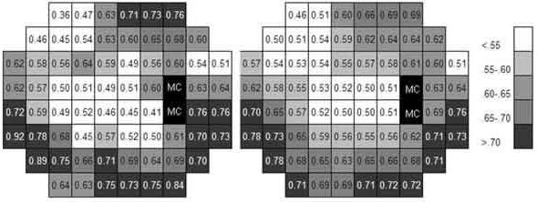
Fig. 3: Left image shows k values calculated at the 66 examined points. In the right image, the average values 
of each area (average of each point and the surrounding) are shown to smooth local differences probably due to procedure errors.
The schemes correspond to the right eye. «BS» corresponds to the blind spot.

Table I shows the average values of the thresholds obtained at the four quadrants of the visual field and the resulting averaged k value. k reached minimum values in the supero-nasal quadrant and maximum values in the lower-nasal quadrant.

The k value increased in a lineal manner from the center towards the periphery, but with different slopes at different meridians. When the relation between the k value and the eccentricity of the 66 points was calculated, a relatively low correlation coefficient was obtained (r= 0.52, p<0.01) due to the different behavior of k at each meridian. However, when the points were grouped on their 10 eccentricity values, k averages reached a high correlation with eccentricity (r=0.98, p<0.01) with a slope of 0.01 per degree (fig. 4).

Fig. 4: Average k values at 10 eccentricity levels in which the 66 examined points are grouped.

When the results obtained with sizes Goldmann 1.9, 2, and 3 were analyzed independently, k values increased in relation to those estimated using the five sizes (fig. 5). On the other hand, when only the results obtained with sizes 3, 3.5 and 4 were used, the k value was reduced. However, the characteristics previously described for the different visual field areas were more or less maintained. The supero-nasal quadrant had the lowest k value, similar to the para-central region.

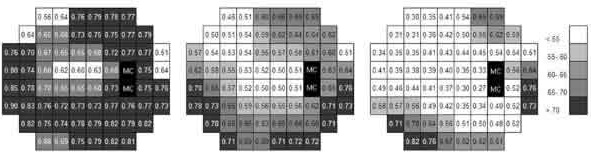
Fig. 5: k values obtained using Goldmann sizes 1.9, 2 and 3 (left) and sizes 3, 3.5 and 4 (right) 
in comparison to the average k values (centre).

Average k values comparable to those described by other authors using commercial perimeters and different mathematical procedures were obtained. The k value’s average increment with eccentricity was also similar to those shown or deduced from other papers (3,7,10-13). Our procedure essentially differs in the mathematical calculation of k and on the strategy for visual field examination, which is adapted for the local dependence characteristics at near points and acts as a local average. Pearson’s variation coefficient applied to the experimental data allows the obtaining of highly congruent results, as can be observed from figures 1 and 2, and allows obtaining of detailed local estimations of spatial summation, which is the main contribution of this paper.

Similar behaviour of spatial summation in the vertical and horizontal meridians (10) and differences in the four meridians being a matter of scale (2) has been described previously. In contrast, our results indicate a very different behaviour of spatial summation in the upper and lower visual fields, probably because those meridians, where k varies most (between 120º and 150º), were not examined in these papers. The topographic changes of normal threshold do not seem to be related to those observed in spatial summation.

If, as described by Galway-Heath (8), the stimulus area can be represented by the number of cells, giving the equation L x A^k=constant, an irregular distribution of these cells would explain the asymmetrical behaviour observed for spatial summation. However, several studies have reported that the lower retina has a lower ganglion cell concentration (14,15) than the upper retina, so that in any case, an increment of the k value in relation to the lower visual field should be expected. However, in our experience, just the opposite happens.

It has been confirmed that k varies with the size range analysed, but topographical differences are maintained relatively constant. Therefore, luminous sensitivity and visual acuity differences between the para-central visual field and some peripheral areas of the upper field which explain cortical magnification (16), are not apparently accompanied by a proportional change in spatial summation. Differential light sensitivity and other physiological parameters degrade towards the periphery with relative dependence on the local ganglion cell density. But in the case of the k value this must not be the only factor involved. We must suppose that, just like in other visual functions, there ought to be variations in ganglion cell physiological characteristics across the retina (17) or other factors that would explain this disparity. Examples are the differences of axon diameter from cells that come from the upper and lower hemi-retinas (18), the opposing differences on A and B horizontal cells (19) or several studies which have found higher cone density in the lower hemi-retina (20,21).

REFERENCES

1. Goldmann H. Grundlagen exakter Perimetrie. Ophthalmologica 1945; 109: 57-70.         [ Links ]

2. Latham K, Whitaker D, Wild JM. Spatial summation of the differential light threshold as a function of visual field location and age. Ophthalmic Physiol Opt 1994; 14: 71-78.         [ Links ]

3. Gougnard L. Étude des summations spatiales chez le sujet normal par la périmétrie statique. Ophthalmologica 1961; 142: 469-486.         [ Links ]

4. Dannheim F, Drance SM. Studies of spatial summation of central retinal areas in normal people of all ages. Can J Ophthalmol 1971; 6: 311-319.         [ Links ]

5. Verriest G, Ortiz-Olmedo A. Étude comparative du seuil différentiel de luminance et de l'exposant de sommation spatiale pour des objets pleins et pour des objets annulaires de mèmes surfaces. Vision Res 1969; 9: 267-282.         [ Links ]

6. Fankhauser F. Problems related to the design of automatic perimeters. Doc Ophthalmol 1979; 47: 89-139.         [ Links ]

7. Gramer E, Kontic D, Krieglstein GK. Die computerperimetrische Darstellung glaukomatoser Gesichtsfelddefekte in Abhangigkeit von der Stimulusgrosse. Ophthalmologica 1981; 183: 162-167.         [ Links ]

8. Garway-Heath DF, Caprioli J, Fitzke FW, Hitchings RA. Scaling the hill of vision: the physiological relationship between light sensitivity and ganglion cell numbers. Invest Ophthalmol Vis Sci 2000; 41: 1774-1782.         [ Links ]

9. Gonzalez de la Rosa M, Martinez A, Sánchez M, Mesa C, Cordoves L, Losada MJ. Accuracy of the Tendency-Oriented Perimetry with the Octopus 1-2-3 Perimeter. In: Wall M, Heijl A. Perimetry Update 1996/1997. Amsterdam: Kugler; 1997; 119-123.         [ Links ]

10. Sloan LL. Area and luminance of test object as variables in examination of the visual field by projection perimetry. Vision Res 1961; 1: 121-138.         [ Links ]

11. Wilson ME. Invariant features of spatial summation with changing locus in the visual field. J Physiol 1970; 207: 611-622.         [ Links ]

12. Wood JM, Wild JM, Drasdo N, Crews SJ. Perimetric profiles and cortical representation. Ophthalmic Res 1986; 18: 301-308.         [ Links ]

13. Kasai N, Takahashi G, Koyama N, Kitahara K. An analysis of spatial summation using a Humphrey field analyzer. In: Mills RP. Perimetry Update 1992/1993. Amsterdam: Kugler; 1992; 557-562.         [ Links ]

14. Curcio CA, Allen KA. Topography of ganglion cells in human retina. J Comp Neurol 1990; 300: 5-25.         [ Links ]

15. Danckert J, Goodale MA. Superior performance for visually guided pointing in the lower visual field. Exp Brain Res 2001; 137: 303-308.         [ Links ]

16. Rovamo J, Virsu V. An estimation and application of the human cortical magnification factor. Exp Brain Res 1979; 37: 495-510.         [ Links ]

17. Wild JM, Wood JM, Flanagan JG. Spatial summation and the cortical magnification of perimetric profiles. Ophthalmologica 1987; 195: 88-96.         [ Links ]

18. Fitzgibbon T, Funke K. Retinal ganglion cell axon diameter spectrum of the cat: mean axon diameter varies according to retinal position. Vis Neurosci 1994; 11: 425-439.         [ Links ]

19. Muller B, Peichl L. Horizontal cells in the cone-dominated tree shrew retina: morphology, photoreceptor contacts, and topographical distribution. J Neurosci 1993; 13: 3628-3646.         [ Links ]

20. Muller B, Peichl L. Topography of cones and rods in the tree shrew retina. J Comp Neurol 1989; 282: 581-594.         [ Links ]

21. Curcio CA, Sloan KR, Kalina RE, Hendrickson AE. Human photoreceptor topography. J Comp Neurol 1990; 292: 497-523.         [ Links ]